Below I provide a comprehensive overview of LVR and AMM design. I cover the following:

• Are AMM LPs profitable? - Results from empirical studies on LP profitability and CEX-DEX arbitrage.
• The LVR Framework - Theoretical results on LVR as introduced in Milonis et. al. 2023 and Milionis, Moallemi & Rougharden 2023.
• AMM Design - Recently proposed LVR mitigation mechanisms.

Are AMM LPs Profitable?

AMM LPs run a market making strategy, taking the other side of every swap executed against the pool. The AMM is constantly quoting a price which is a function of pool reserves with a spread defined by the swap fee.

Since the AMM has no knowledge of external prices, LPs are exposed to adverse selection from informed traders who buy from the pool below fair value and sell to the pool above fair value. The AMM also interacts with uninformed traders, who use the pool as a liquidity source for idiosyncratic reasons. Such swaps are uncorrelated to short-term market moves.

While arbitrage profits extracted from the pool generate losses for LPs, fees generate revenue for LPs. There has been significant interest in figuring out which effect is dominant. If AMMs attract too much toxic flow relative to non-toxic flow, LPs are probably losing money. If AMMs attract sufficient non-toxic flow relative to toxic flow, LPs may be making money.

Measuring LP Profitability

Before quantifying LP profitability, we need to figure out how to measure it. Recent studies use markout PnL. Although markouts are a standard metric used by market making firms, there has been back-and-forth around using them for AMM LPs. The debate is related to the LVR and the empirical LVR section discusses the connection. For now, we motivate markout PnL and compare it to realized PnL.

Let’s start by considering what an ideal PnL measure would be. For a series of $n$ trades, define: $\mathsf{Ideal\; PnL} = \sum_{i = 1}^n \left(P^{\mathsf{fair}}_i - P^{\text{e}}_i\right) q_i s_i$ where $P^{\mathsf{fair}}$ is fair value, $P^{\text{e}}$ is the execution price inclusive of swap fees paid by traders, $q$ is the quantity of the risky token swapped, and $s$ is the side of the trade from the AMM’s perspective (+1 when LPs buy the risky token, -1 when LPs sell).

Each term in ideal PnL captures the AMM’s edge on a trade. It is positive when the AMM buys below fair value or sells above fair value. It is negative, otherwise. So, over a large number of trades, ideal PnL would give a clear picture of whether an AMM profits more in fee income or loses more in adverse selection costs.

Markout PnL

Markout PnL is just ideal PnL with a specific estimate of fair value.

Measuring Fair Value with Pool Prices

Let’s walk through what choices we have to measure fair value. On an AMM, all we see are pool prices. After any given swap, the pool price could be above or below fair value depending on the intentions of the last trader. For example, a degen aping into a new token will push the pool price far above fair value. As a result, markouts estimate fair value as $P^{\mathsf{pool}}({\Delta})$, the pool price time $\Delta$ later. Why is this reasonable? We typically model prices as martingales. So, in expectation, current fair value equals fair value time $\Delta$ later. Also, in expectation, fair value time $\Delta$ later equals the pool price time $\Delta$ later. It follows that $\mathbb{E}\left[P^{\mathsf{pool}}({\Delta})\right] = P^{\mathsf{fair}}$, so we have an unbiased estimator.

Markout Duration

The next question: What is the optimal markout duration $\Delta$? As @0x94305 explains, there is a bias-variance tradeoff. The pool price time $\Delta$ into the future can differ from current fair value just due to long-term market moves. So, if we set $\Delta$ very large, $\mathsf{Var}\left(\lvert P^{\mathsf{pool}}({\Delta}) - P^{\mathsf{fair}} \rvert \right)$ will be large, and markout PnL will be noisy as market risk dominates the AMM’s edge we seek to quantify. If we set $\Delta$ too small, the pool will not have enough time to reverse temporary price impact from uninformed trades. If the last trade was a degen aping into a new token, the pool price is biased upwards. So, $\mathbb{E}\left[\lvert P^{\mathsf{pool}}({\Delta}) - P^{\text{e}}\rvert \right] > \mathbb{E}\left[\lvert P^{\mathsf{fair}} - P^{\text{e}} \rvert \right]$, and we would overestimate the AMM’s edge. Balancing the two effects, we want $\Delta$ to be just large enough for temporary price shocks to disappear. So, the optimal $\Delta$ will depend on the microstructure of a specific AMM pool. In practice, for major Uniswap v3 pools, markouts in the range of 5-10mins are likely optimal. See @0xfbifemboy’s excellent analysis.

Measuring Fair Value with CEX Prices

There is one final improvement to the formulation above. Price discovery for major crypto assets happens on high volume, deep liquidity CEXes such as Binance. Better than pool prices, we should use CEX prices to define fair value. Then, we define markout PnL as: $\mathsf{Markout\; PnL} = \sum_{i = 1}^n \left(P^{\mathsf{CEX}}_i(\Delta) - P^{\text{e}}_i\right) q_i s_i$

Realized PnL (IL + Fees) and Market Noise

Let’s consider realized PnL, aka impermanent loss (IL) plus fees. Sometimes LP performance is evaluated by comparing the final value of the pool assets plus fees to a HODL portfolio, which holds the initial pool assets instead of depositing into the AMM. Say we have an ETH/USDC pool. Then, we can calculate realized PnL as: $\mathsf{Realized\; PnL} = y_n - y_0 + P^{\mathsf{pool}}_n (x_n - x_0) + \mathsf{fees}_n$ where $y_i$ are the USDC reserves, $x_i$ is the are ETH reserves, $\mathsf{fees}_i$ is the value of accrued fees and $P^{\mathsf{pool}}_i$ is the pool price at trade $i$.

What is strange about realized PnL? Assume that swap fees are small, so $\mathsf{fees}_n \approx 0$. Then, realized PnL is 0 whenever the initial and final ETH price are equal. A CPMM’s reserves fully determine the pool price. So, when $P^{\mathsf{pool}}_0 = P^{\mathsf{pool}}_n$, it follows $y_0 = y_n$ and $x_0 = x_n$.

Concretely, imagine two cases with realized PnLs of 0. In the first case, pool prices move 1000 $\rightarrow$ 4000 $\rightarrow$ 1000. In the second case, the pool price holds steady at 1000. Intuitively, one would expect these numbers to be different. Volatility and hence arbitrage trades in the first case should imply lower LP PnL numbers. The issue is that realized PnL merely takes a snapshot of the AMM and HODL portfolios at start and finish. It ignores the trajectory of ETH prices and trades in the middle, so effectively all that matters is where the ETH price ends up. It suffers from the same problem as setting $\Delta$ too high in markouts: market noise creates too much variance.

Markout PnL and Market Noise

To see why markout PnL eliminates the effect of market noise, lets re-write the formula, as suggested by @AnthonyLeeZhang : $\begin{aligned} \mathsf{Markout\; PnL} = \underbrace{\sum_{i = 1} ^n P^{\mathsf{CEX}}_i(\Delta) q_{i} s_{i}}_{\mathsf{Hedge\; PnL}} + \underbrace{\sum_{i = 1}^n P^{\text{e}}_{i} q_{i} (-s_{i})}_{\mathsf{AMM\; PnL}} \end{aligned}$ The AMM PnL term is what the AMM makes over the course of its trades. The hedge PnL term is what you would make doing the opposite of the AMM’s trades on a CEX time $\Delta$ into the future (assuming the CEX has no fees and infinite liquidity). Hence markout PnL is the PnL of a delta-hedged strategy where the frequency of the hedge is determined by $\Delta$. By delta-hedging, we eliminate the effect of moves in market prices.

This decomposition also implies that, in expectation, markout PnL is equivalent to realized PnL. The hedge trades on the CEX at fair value. Since prices are martingales, no one should have any edge on the market executing at fair value. So, $\mathbb{E}[\mathsf{Hedge\; PNL}] = 0$. We can also re-write AMM PnL directly in terms of the change in the pool’s value plus accrued fees. Using the martingale property of prices again and summing terms up, we conclude: $\begin{aligned} \mathbb{E}\left[\mathsf{Markout\; PnL}\right] &= \mathbb{E}\left[y_n - y_0 + P^{\mathsf{pool}}_nx_n - P^{\mathsf{pool}}_0 x_0 + \mathsf{fees}_n\right] \\ &= \mathbb{E}\left[y_n - y_0 + P^{\mathsf{pool}}_nx_n - P^{\mathsf{pool}}_0 x_0 + \left(P^{\mathsf{pool}}_0 - P^{\mathsf{pool}}_n\right)x_0 + \mathsf{fees}_n\right]= \mathbb{E}\left[\mathsf{Realized\;PnL}\right]\\ \end{aligned}$

Markout PnL as a Measure for Expected LP Profitability

In conclusion, markout PnL tells us much more about expected LP profitability compared to realized PnL. LP performance is the sum of the AMM’s market making edge and mean zero market noise. By eliminating the latter and focusing in on the former, it delivers lower variance estimates.

Empirical PnL Studies

Uniswap v3 ETH/USDC

@thiccythot_ conducted the first markout PnL study of LPs across all Uniswap v3 ETH/USDC pools. @0xfbifemboy did a follow-up analysis.

The major result is that between Aug 2021 and Nov 2022, aggregate 5-minute markout PnL is approximately -$40 million.

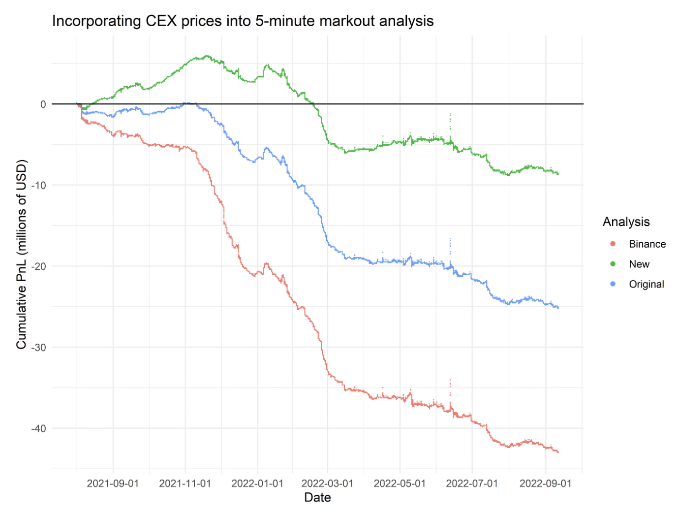
There are a few important conclusions from @0xfbifemboy’s follow-up study.

• Downwards bias in original study: @thiccythot_’s original study shows PnLs as large as -$100 million for 24-hour markouts. However, the study likely underestimates PnL because it estimates fair value with $P^{\text{e}}(\Delta)$, the execution price closest to time $\Delta$ into the future, instead of the pool price. Execution prices include fees. When you diff two execution prices resulting from swaps in the same direction, the fee cancels out and PnLs look worse. When you diff execution prices from swaps in opposite directions, you double count the fee. However, the first effect is dominant since swap directions tend to be autocorrelated. See “Original” vs “New” in the graph above to compare how the 5-minute markouts change.
• Binance markouts: When you use $P^{\mathsf{CEX}}(\Delta)$ instead of $P^{\mathsf{pool}}(\Delta)$, PnLs are negative across all fee tiers and across all markout durations 5 minutes or longer. Binance markouts are more pessimistic about LP PnL than pool price markouts. See “New” vs “Binance” in graph above.
• 0.05% pool performance: The 0.05% fee tier is extremely unprofitable. LPs in the 0.3% pool perform better across a variety of metrics. As the graph below shows, even if you set $\Delta$ to 0, which should vastly overestimate PnL, the 0.05% pool loses money. Given the 0.05% pool dominates swap volume, it drives most of the aggregate LP losses. 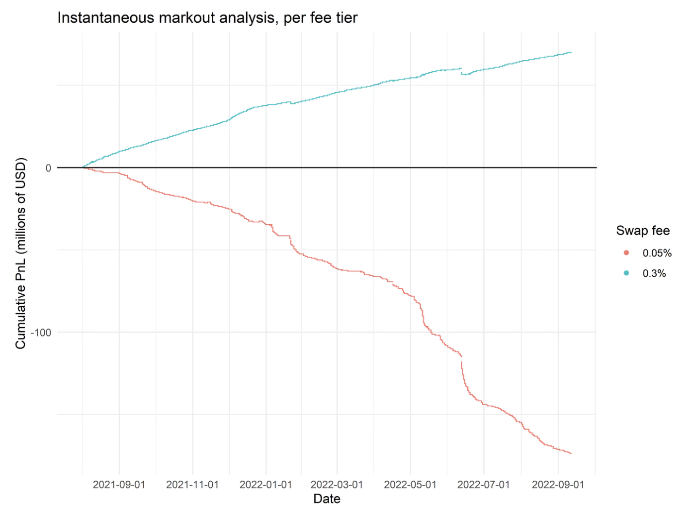Other studies generally confirm the markout analysis. Realized PnL for closed LP positions in the 0.05% pool generated -$67 million between Aug 2021 and Sep 2022. Note that only analyzing closed positions is tricky; it means the PnL estimate may be upwards biased due to the disposition effect.

Uniswap v2 ETH/USDC

Milonis et. al. 2023 run an empirical study of LP profitability for the Uniswap v2 ETH/USDC pool.

Between Aug 2021 and Aug 2022, 5-minute delta-hedged PnL is around +$17 million. Delta-hedged PnL is quite similar to Binance-based markout PnL.

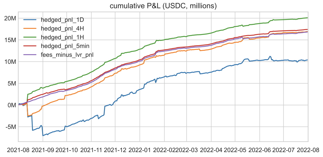
Lower gas and more non-toxic flow in v2 compared to v3 might drive its positive profitability.

Other Chains

@0xfbifemboy has an analysis covering Uniswap v3 ETH/USDC pools on Polygon. Swaps occur at a higher frequency and tend to be smaller than Ethereum mainnet. When comparing liquidity-normalized markout PnL, LPs do ~10-20% better on average. Finally, just like Ethereum, the 0.3% fee tier outperforms the 0.05% fee tier.

Other Pools

There are limited studies on pools aside from ETH/USDC. Loesch et. al. 2021 conducted an analysis of realized PnL across a wider range of major Uniswap v3 pools, covering 43% of TVL. In aggregate, PnL was -$60 million between May and Sep 2021. Due to how skewed Uniswap TVL is towards major pools, this headline number largely reflect PnLs from the largest pools. However, the effect is fairly consistent: 15 out of 17 pools experienced negative PnL. 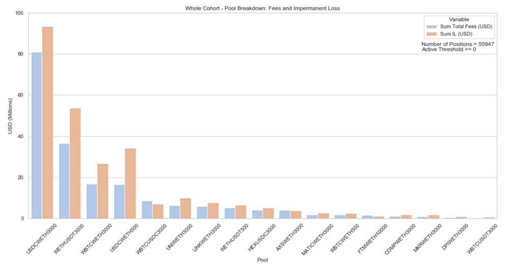Despite the lack of published numbers, one-off analyses point to the following breakdown: Realized PnL tends to be negative for major assets, can be positive for pegged pairs, and can be positive for stable pairs (assuming the peg holds in your sample). Long-tail assets behave differently and it can be profitable to LP in those pools.

CEX-DEX Arbitrage

Who is on the other side of LP losses? Informed traders, specifically stat arb teams engaging in CEX-DEX arbitrage.

CEX order books update at millisecond frequencies, while Ethereum state only updates every 12 seconds with the arrival of a new block. Between blocks, AMM LPs are stuck quoting a stale price as the CEX price moves around. When the dislocation is large enough, stat arb teams trade on the AMM until its reaches the CEX price and hedge that position on a CEX. The arbitrageur profits come out of the pockets of LPs.

To understand the mechanics and economics of CEX-DEX arbitrage, we can take a look at some data on Ethereum blocks and the MEV boost auction (responsible for +90% of Ethereum blocks).

Bidding for Top-of-Block Access

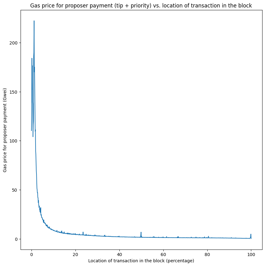
Ethereum blocks currently tend to delineate between the top-of-block (TOB) and rest-of-block (ROB). As shown in @ankitchiplunkar’s analysis, gas prices for transactions in the first 5-10% of the block are two orders of magnitude higher than the remainder of the block. The TOB comprises state contentious activities, while the ROB comprises everything else. CEX-DEX transactions are always in the TOB as stat arb teams need first touch access to AMM pools and are willing to bid aggressively for that right.

Increasingly, stat arb teams run builders and pay large MEV-boost bribes to guarantee themselves TOB access. As a concrete example, consider block 17195495 where a builder paid the proposer ~17 ETH. Gupta, Pai & Resnick 2023 explain how the TOB was all CEX-DEX transactions:

CEX/DEX arb transactions are easily identifiable since they are large directional trades, typically in the first few slots of the block.

These CEX/DEX arb transactions are usually executed by an MEV bot contract that disproportionately lands transactions in blocks associated with the corresponding builder. For example, block 17195495 contains 182 transactions. The first 37 appear to be CEX/DEX arb transactions from an MEV bot with the address 0xA69b…e78C. These are subjectively large swaps on major pools (uniswap, sushiswap etc). For example, the first transaction swaps 4.265 Million USDC for 2168 wETH on the Uniswap v3 0.05% fee pool. The subsequent 36 are also similarly large swaps, each of the order of several hundred wETH.

The SMG team also has an excellent visualization of how builder bids and Binance prices moved together over the duration of this slot.

Estimating the Value of CEX-DEX Arbitrage

It is difficult to calculate the value of CEX-DEX arbitrage given we can only see the on-chain leg of trades, but a rough estimate can give us a sense how much LP lose to toxic flow across all major pools.

In the following piece, the Frontier Research team found that around 16% of all proposer payments are from CEX-DEX transactions in a four month period following the merge. This number is conservative since the team was careful to avoid false positives when identifying CEX-DEX transactions. 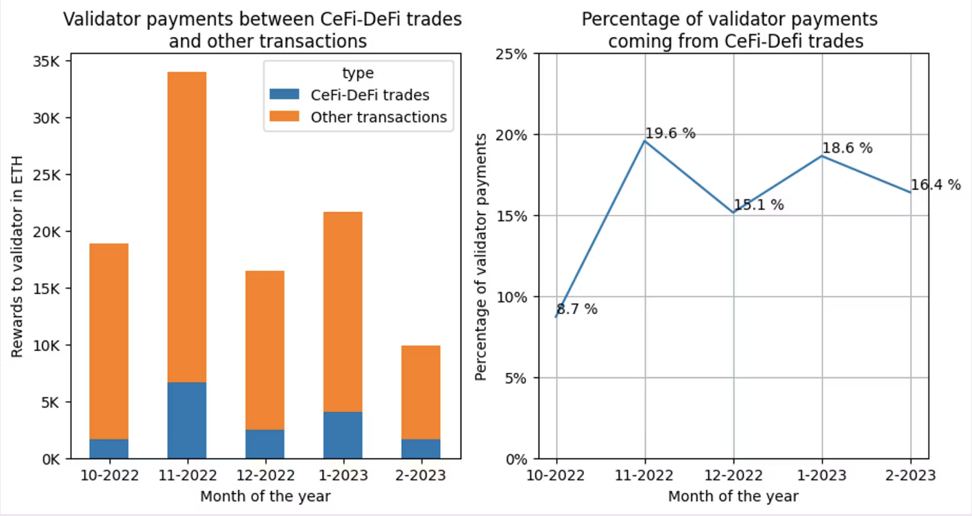About $544 million/year are paid through MEV-boost currently. Applying the 16% number, we get a lower bound of $87 million/year paid by CEX-DEX arbitrageurs to proposers. In another Frontier Research post, the authors suggest stat arb teams pay 37-77% of revenue to proposers, implying total revenue of 112 to 235 million/year. They also run a more granular, trade by trade markout analysis, where they find CEX-DEX revenue in Q1 2023 was 37.8 million. This is also a lower bound number since their dataset only captured ~80% of all relevant trades.

Identifying the Players

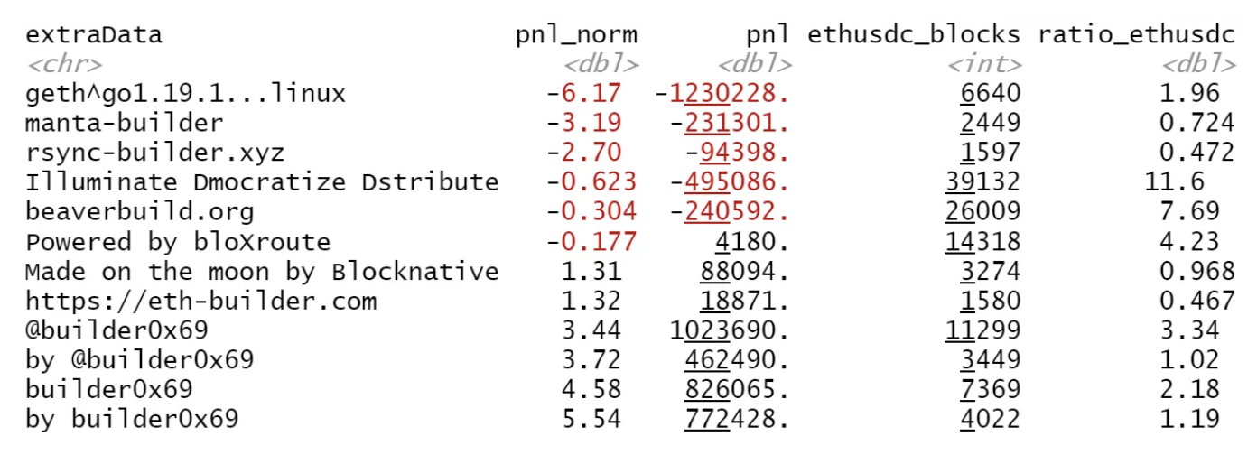
CEX-DEX arbitrage is dominated by a small set of sophisticated players. Gupta, Pai & Resnick 2023 identify three “HFT builders” (beaverbuild, manta-builder, rsync-builder) and estimate how likely they are to win a block given 12-second volatility on Binance. The model shows that when prices are flat, they win with probability 30%. When volatility is 1%, they win with probability 77.5%. When volatility is 2%, they win with probability 97%.

The result matches 0xfbifemboy’s analysis which shows that the majority of toxic flow in Uniswap pools comes from specific builders. From Sep 2022 to March 2023, manta-builder, generated -1.2 million in PnL for ETH/USDC LPs. This is striking given they constructed less than 3% of the blocks with ETH/USDC swaps, and LPs actually made 1 million in PnL over this period.

The LVR Framework

Loss-Versus-Rebalancing (LVR) is formulated in Milonis et. al. 2023 as a way to think about adverse selection costs suffered by LPs in the face of arbitrageurs. It is defined as the performance gap between an LP position and a rebalancing strategy, which replicates the AMM trades but executes them at CEX prices. LVR reveals the source of LP losses is price slippage: the AMM executes trades at prices worse than CEX prices. Practically, one should interpret LVR as arising from trades made by the AMM with informed traders who arbitrage stale AMM prices against CEX prices.

Empirical LVR

It is best to start with empirical LVR, an ex-post metric which measures LP losses given historical data.

Consider the example covered in Tim Rougharden’s talk.

We LP into a ETH/USDC Uniswap v2 pool, depositing 1 ETH and 1000 USDC. Now, we track what happens over the next 2 time periods as the CEX price moves:

• $\mathbf{t_0}$: The CEX price is 1000. The pool price is also 1000 since it is the ratio of the reserves, 1000/1.
• $\mathbf{t_0 \rightarrow t_1}$: The CEX price moves to 4000. The AMM sells 0.5 ETH and buys 1000 USDC from arbitrageurs, setting the ratio of reserves 2000/0.5 = 4000. The AMM executed at a price of 1000/0.5 = 2000.
• $\mathbf{t_{1}}$: Both CEX and pool prices are 4000.
• $\mathbf{t_1 \rightarrow t_2}$: The CEX price moves to 1000. The AMM buys 0.5 ETH and sells 1000 USDC to arbitrageurs, setting the ratio of reserves 1000/1 = 1000. The AMM executed at a price of 1000/0.5 = 2000.
• $\mathbf{t_{2}}$: Both CEX and pool prices are 1000.

What is the rebalancing strategy? Imagine someone who also starts with 1 ETH and 1000 USDC. Then, they copy trade the AMM, but always execute on the CEX. In $t_0 \rightarrow t_1$, they sell 0.5 ETH at price of 4000. In $t_1 \rightarrow t_2$, they buy 0.5 ETH at a price of 1000.

For a sequence of $n$ AMM trades, we define empirical LVR as: $\mathsf{Empirical\; LVR} = -\sum_{i = 1}^{n} \left(P^{\mathsf{CEX}}_{i} - P^{\mathsf{pool}}_{i}\right)q_{i} s_{i}$ where $P^{\mathsf{CEX}}$ is the CEX price, $P^{\mathsf{pool}}$ is the AMM price and $q_i$ and $s_i$ as defined in the same way as markout PnL.

In our example, empirical LVR works out to 1000 + 500 = 1500. In $t_{0} \rightarrow t_{1}$, both strategies sell 0.5 ETH, but the AMM executes at a price 2000 lower than the rebalancing portfolio, creating a performance gap of 1000. In $t_{1} \rightarrow t_{2}$, both strategies buy 0.5 ETH, but the AMM executes at a price 1000 higher than the rebalancing portfolio, creating a performance gap of 500. When you add everything up, empirical LVR comes out precisely to the difference in the final portfolio values, 3500 - 2000 = 1500.

Markout PnL = Fees - Empirical LVR

Inspecting the formula, we see that the negative empirical LVR has the same form as markout PNL, but $P^{\mathsf{fair}}$ is estimated as $P^{\mathsf{CEX}}$ (setting $\Delta$ = 0) and execution price $P^{\text{e}}$ is replaced with $P^{\mathsf{pool}}$. Since the difference between execution and pool prices is fees, it follows that markout PnL is just fees minus empirical LVR.

Given this relationship, empirical LVR inherits the nice properties of markout PnL. It cleanly captures the idea of adverse selection costs faced by LPs in the face of arbitrageurs by evaluating performance on a trade-by-trade basis. Unlike IL, it is path-dependent and eliminates the effect of market noise. Further, because it ignores fees and only focuses on LP losses to arbitrage, it is guaranteed to be non-negative and non-decreasing.

Ex-Ante LVR

Ex-ante LVR is a formal model which precisely characterizes what factors drive LP losses under Black-Scholes style assumptions.

It is important to keep in mind that ex-ante LVR provides a theoretical upper bound on arbitrage profits that can extracted at the expense of LPs. The model ignores swap fees, discrete block times and gas costs, all of which limit arbitrage profits. In the next section, we will add these features to the model.

Assumptions

There is a risky asset $x$ and a numéraire asset $y$. The risky asset can be traded with zero fees on a CEX with infinite liquidity. The CEX price is exogenous and governed by geometric Brownian motion (GBM) with stochastic volatility.

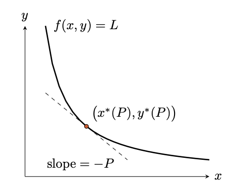
There is an AMM with reserves $(x, y)$ of the risky and numéraire assets. The AMM is defined by a bonding curve $f(x, y) = L$, with liquidity held constant.

There are two types of agents:

• LPs, who have deposited assets to the AMM. They are completely passive, so they do not mint or burn liquidity.
• Arbitrageurs, who trade frictionlessly on the CEX and are continuously monitoring the AMM price to exploit any deviation from the CEX price. If arbitrageurs observe the CEX price $P$, they will move the AMM reserves to a point along $f(x, y)$ where the slope of the curve is $-P$. They pay no fees on the AMM.

The set-up also ignores any details of the underlying blockchain: there are no gas fees and no discrete block times.

Value of the AMM Reserves

The value of the AMM reserves is defined by the pool value function: $\begin{aligned} V(P) \triangleq & \quad \min_{(x, y) \in \mathbb{R}^2_{+}} & \quad Px + y \\ &\quad \text{subject to} & \quad f(x, y) = L \\ \end{aligned}$ Intuitively, this optimization follows from recognizing that:

1. Arbitrage profits are maximized by minimizing the market value of the AMM reserves, $Px + y$.
2. Arbitrageurs are always able to trade with the AMM in a way that obeys the bonding curve, $f(x, y) = L$.

So, the existence of arbitrageurs implies that the value of AMM reserves at any time $t$ is given by $V_t = P_t x_t + y_t$ where $x_t = x^{\ast}(P_t)$, $y_t = y^{\ast}(P_t)$, and $(x^{\ast}(P_t), y^{\ast}(P_t))$ is optimal solution to the pool value function.

Since LPs own shares of the AMM reserves, their PnL is simply: $\mathsf{LP\,PnL}_{t} = V_{t} - V_{0} + \mathsf{FEE}_{t}$ In other words, LP PnL is the change in the value of the AMM reserves plus the cumulative value of fees earned.

Value of the Rebalancing Strategy

The rebalancing strategy replicates the AMM reserves at each point-in-time. It buys and sells the same amount of the risky asset as the AMM, but executes at CEX prices. More precisely, the rebalancing strategy begins holding $(x^{\ast}(P_0), y^{\ast}(P_0))$, the initial AMM portfolio. Then, it continuously and frictionlessly trades on a CEX to maintain a position in the risky asset given by $x_{t} \triangleq x^{*}(P_t)$.

If, we denote the value of the rebalancing portfolio as $R_{t}$, the rebalancing PnL is: $\mathsf{Rebalancing\, PnL}_{t} = R_{t} - V_{0} = \int_{0}^{t} x^{*}(P_s)dP_s$ The rebalancing portfolio starts at the same value as the AMM pool, $V_0$. Since all of its trades execute exactly at the CEX price, they have zero effect on the strategy’s profit. Recall no can have edge against the market executing at fair value. So, the PnL is simply the integral of instantaneous holdings of the risky asset, $x^{*}(P_s)$, times the change in price, $dP_s$.

Finally, note that due to equivalent holdings in the risky asset, a long position in the AMM LP and short position in the rebalancing strategy would delta-hedge one’s exposure to moves in the risky asset’s price.

Defining Ex-Ante LVR

We define LVR as the difference in the value of rebalancing strategy and value of the AMM reserves: $\mathsf{LVR}_{t} \triangleq R_t - V_t$ The crucial theorem in the paper is as follows. LVR takes the form: $\mathsf{LVR}_{t} = \int_{0}^t \ell(\sigma_s, P_s) ds \quad\quad \text{where} \quad\quad \ell(\sigma, P) \triangleq \left| x^{\ast \prime}(P) \right| \frac{\sigma^2P^2}{2} \geq 0$ Further, we have that:

• $\mathsf{LVR}_{t}$ is non-negative and non-decreasing.
• The cumulative profit of arbitrageurs up to time $t$ is $\mathsf{LVR}_{t}$.

Proof Sketch

As a quick proof sketch, consider a ETH-USDC Uniswap v2 pool.

The ETH price on Binance increases from $P_t$ to $P_t + dP_t$. What happens in the AMM? The AMM sells $dx_{t}$ ETH to arbitrageurs, trading along the purple line. It moves from point $A$ (where the red tangency line has slope $P_t$) to point $B$ (where the brown tangency line has slope $P_t + dP_t$). What happens in the rebalancing strategy? The rebalancing strategy also sells $dx_t$ ETH, but it executes at the Binance price of $P_t + dP_t$. Hence it trades moves from point $A$ to point $B^{\ast}$.

Although the AMM and rebalancing strategy sell the same amount of ETH, the rebalancing strategy ends up with more of the numéraire asset. The difference, $B^{*} - B$, is precisely instantaneous LVR. 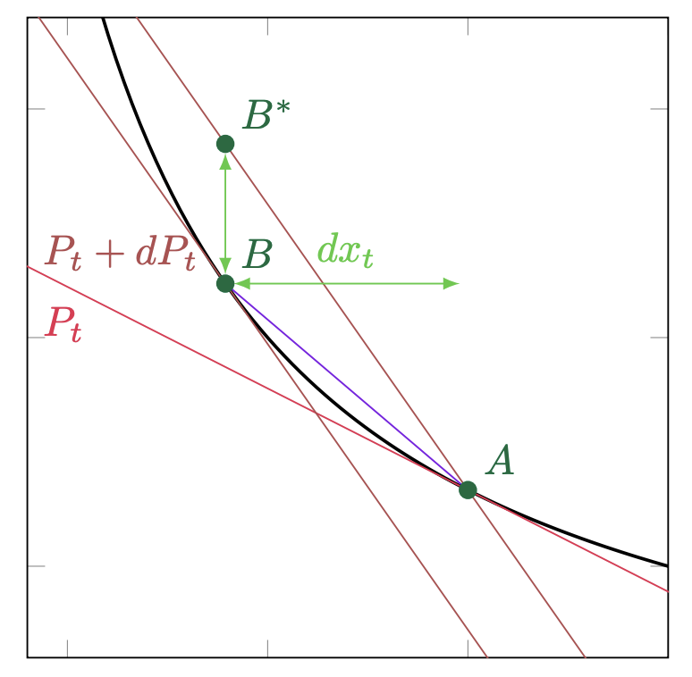More mathematically:

• Given the slopes of the tangent lines at $A$ and $B$, the purple secant line has a slope of $P_t + \frac{dP_t}{2}$.
• The difference $B^{*} - B$ works out to:

$dx_t\left((P_t + dP_t) - \left(P_t + \frac{dP_t}{2}\right)\right) = \frac{dx_t dP_t}{2}$

• The amount traded $dx_t$ can be written as a function of the optimal solution to the pool value function:

$dx_t = \left| x^{\ast \prime}(P_t) \right| dP_t$

• Under the GBM assumption, quadratic variation is given by $(dP_t)^2 = \sigma_{t}^2P_t^2$.
• Combining these results, we conclude instantaneous LVR is:

$\left| x^{\ast \prime}(P_t) \right| \frac{\sigma_{t}^2P_t^2}{2}$

There are two major takeaways from the proof sketch:

1. LVR can be equivalently described as both the loss of the AMM relative to the rebalancing strategy, and arbitrage profits. Arbitrageurs purchase $dx_{t}$ ETH from the AMM at a price of $P_{t} + (dP_{t}/2)$ and sell it on the CEX at a price $P_{t} + dP_{t}$, netting a profit of $(dx_t dP_t)/2$.
2. LVR only depends on two parameters:
   • Volatility, $\sigma_t$
   • Marginal liquidity of the AMM, $\left| x^{\ast \prime}(P_t) \right|$. This value depends on the local convexity of the AMM’s bonding curve. Precisely, it is the slope of the AMM’s demand function for the risky asset at the current pool price. Flatter bonding curves offer higher marginal liquidity. For more details, check out Angeris, Evans, & Chitra 2021.

Interpreting Ex-Ante LVR and LP PnL

From the paper:

The core intuition is that the CFMM systematically loses money relative to the rebalancing strategy due to price slippage: every trade made by the CFMM is made at slightly worse prices than the rebalancing strategy.

Passive LPs are unable to update their prices in response to changes in CEX prices and rely on the arbitrageurs to fix stale prices on the AMM. Since trades on the AMM are zero-sum, any arbitrage profits show up as LP losses.

LVR’s dependence on volatility and marginal liquidity intuitively makes sense. We expect LP losses to arbitrage are larger when prices move around aggressively and when the AMM is willing to trade in larger size for a small change in price.

The LVR result also matches a well-known proof that the static replication of a CPMM LP, ignoring fees, is short a bundle of European options. Since the value and size of the replicating portfolio grows with volatility and the AMM’s marginal liquidity, LVR does as well. Although the short vol interpretation of an LP position is useful, there are some caveats to that line of thinking.

Finally, consider going long the AMM LP and short the rebalancing strategy: $\begin{aligned} \mathsf{hedged\, LP\, PnL}_{t} &= V_{t} - V_{0} + \mathsf{FEE}_{t} - \mathsf{Rebalancing\, PnL}_{t}\\ &= \mathsf{FEE}_{t} - \left(R_{t} - V_{t}\right)\\ &= \mathsf{FEE}_{t} - \mathsf{LVR}_{t} \end{aligned}$ Eliminating the effect of market risk, we see that hedged LP PnL is a balancing act between profits from fee income and losses from LVR.

Ex-Ante LVR for a CPMM and Concentrated Liquidity

For a CPMM, we can derive a closed-form solution for the instantaneous LVR normalized per dollar of pool reserves: $\frac{\ell(\sigma, P)}{V(P)} = \frac{\sigma^{2}}{8}$ For a pool where daily $\sigma = 5\%$, the LPs lose around 3.125 bps in pool value daily to LVR.

Now, consider a concentrated LP position on an AMM like Uniswap v3 with a range $[P_a, P_b]$. When the pool price is in range, instantaneous LVR $\ell(\sigma, P)$ equals the CPMM case. However, the pool value function $V(P) \rightarrow 0$ as $P_a \rightarrow P$ and $P_b \rightarrow P$. So, we have: $\lim_{\substack{P_a \rightarrow P \\ P_b \rightarrow P}} \frac{\ell(\sigma, P)}{V(P)} = + \infty$

Ex-Ante LVR as the “Minimum Variance, Unbiased Measure” of LP Performance

Other LP performance measures consider benchmarks different from the rebalancing strategy.

We will define loss-versus-benchmark as $\mathsf{LVB}_{t} \triangleq \overline{R}_t - V_t$, where $\bar{R}_t$ is the value of any strategy that begins holding the AMM’s initial portfolio and executes at CEX prices. Let $\bar{x}_{t}$ be the strategy’s risky asset holdings. For example, the benchmark in IL calculations is the HODL portfolio, $\bar{x}_{t} = x^{\ast}(P_0)$, so we have: $\mathsf{LVB}_{t}^{\text{IL}} \triangleq R_{t}^{\text{IL}} - V_{t} = V_0 + x^{\ast}(P_0)\left(P_t - P_0\right) - V_{t}$

The key advantage of LVR is that it uniquely eliminates noise from market risk. We can write: $\mathsf{LVB}_{t} = \mathsf{LVR}_{t} + \int_{0}^{t} [\bar{x}_s - x^{*}(P_s)] dP_s$ So, LVB is equivalent to LVR plus a term which represents the difference in the benchmark and AMM risky asset holdings. This second term is mean zero, because any strategy executing at CEX prices cannot beat the market. However, it does have positive quadratic variation. So, $\mathbb{E}[\mathsf{LVB}_{t}] = \mathbb{E}[\mathsf{LVR}_{t}]$, but $[\mathsf{LVB}]_{t} \geq [\mathsf{LVR}]_{t} = 0$.

In conclusion, LVB and LVR theoretically should give the same picture of LP performance over a large number of price paths. But on any specific price path $P_t$, a benchmark may under or outperform the AMM due to differences in holdings of the risky asset. Only the rebalancing strategy always outperforms the AMM. Hence LVR uniquely isolates LP losses from price slippage.

LP Losses Accounting for Fees and Block Times

The original LVR paper is in continuous time and assumes arbitrageurs pay no swap fees. Milionis, Moallemi & Rougharden 2023 model LP losses in AMMs accounting for discrete block times and fees.

Assumptions

The set-up is largely the same, but with two key differences. First, there is an AMM fee of $\gamma$ denoted in units of log price. So, when an agent trades $\Delta y$ of the numéraire asset on the AMM, the fee charged is: $(e^{\gamma} - 1)|\Delta y|$ Second, arbitrageurs can only trade on the AMM at arrival times governed by a Poisson process with a rate $\lambda > 0$. So, the mean block time is $\Delta t \triangleq \lambda^{-1}$.

Arbitrageurs are assumed to myopically maximize immediate profit at arrival times. If the AMM price net of fees is below the CEX price, they buy from the AMM and sell to the CEX until the net AMM price equals the CEX price.

Mispricing Process

Let $\tilde{P}_t$ be the AMM price and $P_t$ be the CEX price. The log mispricing of the pool is given by: $z_t \triangleq \log{P_t/\tilde{P}_t}$ such that $\tilde{P}_t = P_te^{-z_t}$. Now, consider an arbitrageur who arrives at time $t$ and observes AMM price $\tilde{P}_{t^{-}}$ and CEX price $P_{t}$, or equivalently mispricing $z_{t^{-}}$. There are three cases:

1. $z_{t^{-}} > \gamma$, so the CEX price exceeds the AMM price net fees. They will profitably buy from the AMM and sell on the CEX until $z_{t} = \gamma$.
2. $z_{t^{-}} < -\gamma$, so the AMM price net fees exceeds the CEX price. They will profitably buy from the CEX and sell on the AMM until $z_{t} = -\gamma$.
3. $-\gamma \leq z_{t^{-}} \leq \gamma$. They will make no trade, so $z_{t} = z_{t^{-}}$.

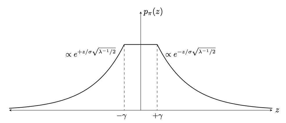
It follows that at arrival times $\tau$, the mispricing process follows: $z_{\tau} = \text{bound}\{z_{\tau^{-}}, -\gamma, +\gamma\}$ For non-arrival times, the mispricing process is governed by the GBM. All together, it is a jump diffusion process. The graph below shows an example path where the red ticks on the x-axis are arrival times. Notice how it jumps into the no-trade region at those ticks. 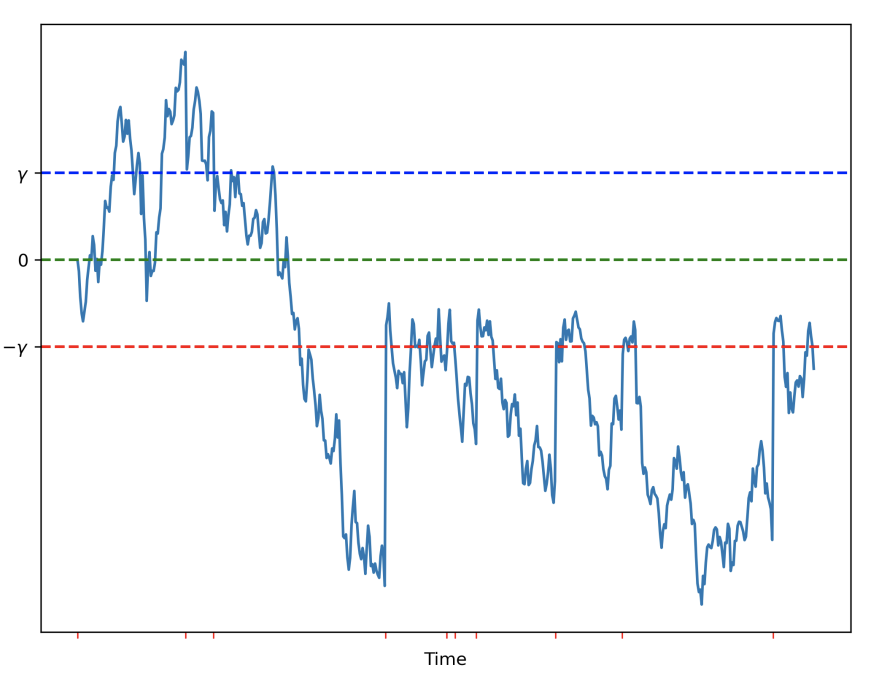The authors derive the stationary distribution of this process. As shown below, it decays exponentially outside the no-trade region, $[-\gamma, \gamma]$, as arbitrageurs will tend to bring the price back inside the no-trade region.

Probability of an Arbitrage Trade

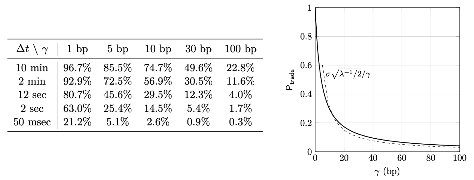
From the distribution above, the probability the mispricing process is outside of the no-trade region can be calculated as: $\mathsf{P_{trade}} = \frac{1}{1 + \frac{\gamma}{\sigma \sqrt{\Delta t/2}}} = \frac{1}{1 + \eta}$ where $\eta \triangleq \gamma / (\sigma \sqrt{\Delta t/2})$, the fee measured as a multiple of the typical movement of returns over half the block time. It is useful to interpret $\mathsf{P_{trade}}$ as the fraction of blocks with a profitable arbitrage trade.

The key takeaways:

• The only AMM property which matters is the fee. The bonding curve does not show up in the formula.
• $\eta$ is large when fees are high, volatility is low and blocks are fast. In that case, the width of the no-trade region is large relative to intrablock price moves, so the mispricing process is less likely to exit the no-trade region. In those regimes, we have $\mathsf{P_{trade}} \approx \eta^{-1}$.

The table below shows values of $\mathsf{P_{trade}}$ for various values of $\Delta t$ and $\gamma$ with when $\sigma = 5\%$ daily. The graph shows a similar result when $\Delta t = 12$ seconds.

Rate of Arbitrage Profit for a CPMM

Given the distribution of the mispricing process and model of arbitrageur behavior, one can derive the rate of instantaneous expected arbitrage profit and fees, defined as $\overline{\mathsf{ARB}} \triangleq \lim_{T \rightarrow 0} \mathbb{E}[\mathsf{ARB}_{T}]/T$ and $\overline{\mathsf{FEE}} \triangleq \lim_{T \rightarrow 0} \mathbb{E}[\mathsf{FEE}_{T}]/T$, respectively. Here $\mathsf{ARB}_T$ and $\mathsf{FEE}_{T}$ are the cumulative arbitrage profits and fees paid through time $T$. The expectation is taken over the distribution of the mispricing process.

The general solutions for $\overline{\mathsf{ARB}}$ and $\overline{\mathsf{FEE}}$ depend on the bonding curve and the marginal liquidity of the AMM. For this point on, we will consider a CPMM, where it is possible to derive an explicit closed form.

Recall the LVR paper establishes that for a CPMM in a continuous time and no fee setting, we know that $\overline{\mathsf{LVR}} = \sigma^{2} V(P)/ 8$. Then, it is possible to derive the rate of arbitrage profit with reference to LVR: $\overline{\mathsf{ARB}} = \overline{\mathsf{LVR}} \times \mathsf{P_{trade}} \times \underbrace{\frac{e^{\gamma /2} + e^{-\gamma/2}}{2}}_{1 + O(\gamma^2)} \times \underbrace{\frac{1}{1 - (\sigma^{2}\Delta t)/8}}_{1 + O(\Delta t)}$ This expression depends on a mild, not practically relevant, technical condition that block times are sufficiently fast relative to volatility: $\Delta t < 8/\sigma^{2}$. Assuming $\sigma = 5\%$ daily, the inequality holds for block times shorter than 3200 days.

The result simplifies considerably in the small fee, fast block regime ($\gamma \rightarrow 0, \Delta t \rightarrow 0$). Specifically, we can approximate: $\begin{aligned} \overline{\mathsf{ARB}} &\approx \overline{\mathsf{LVR}} \times \mathsf{P_{trade}}\\ \overline{\mathsf{FEE}} &\approx \overline{\mathsf{LVR}} \times \left(1 - \mathsf{P_{trade}}\right) \end{aligned}$ These approximations are extremely accurate for practical values of $\gamma$ and $\Delta t$. The graph below shows the size of the error when $\sigma = 5\%$ daily and $\Delta t = 12$ seconds.

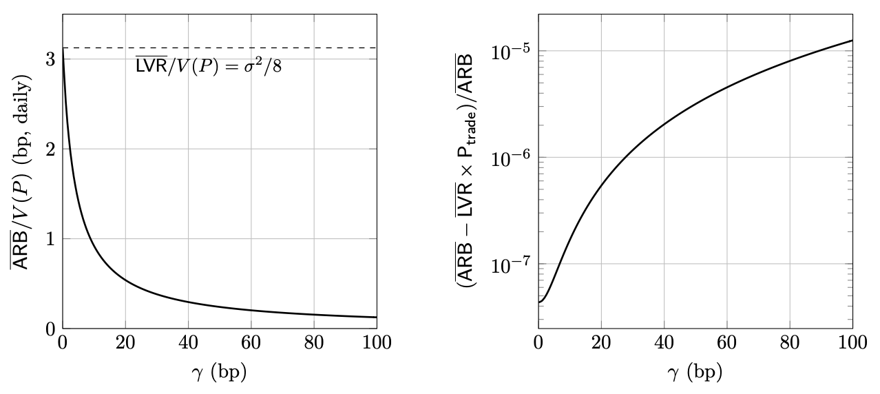
Interpreting $\overline{\mathsf{ARB}}$ and $\overline{\mathsf{FEE}}$

We have shown a very nice breakdown $\overline{\mathsf{ARB}} + \overline{\mathsf{FEE}} \approx \overline{\mathsf{LVR}}$. LVR is split between arbitrage profits and LP fees as governed by $\mathsf{P_{trade}}$. As we make block times faster, the the fraction of blocks with a profitable arbitrage trade decreases, so more and more LVR is captured as fees.

Plugging in formulas for $\overline{\mathsf{LVR}}$ and $\mathsf{P_{trade}} \approx \eta^{-1}$, we can see how arbitrage profits scales with key parameters in the small fee, fast block regime: $\overline{\mathsf{ARB}} = \mathsf{const} \times \frac{\sigma^{3}}{\gamma}\sqrt{\Delta t} + o\left(\sqrt{\Delta t}\right)$ It is proportional to square root of block time, cube of volatility, and reciprocal of the fee.

@0x94305 provides a nice proof sketch of the formula:

• Under the GBM assumption, the CEX price makes random moves of size $\sigma \sqrt{\Delta t}$ between blocks.
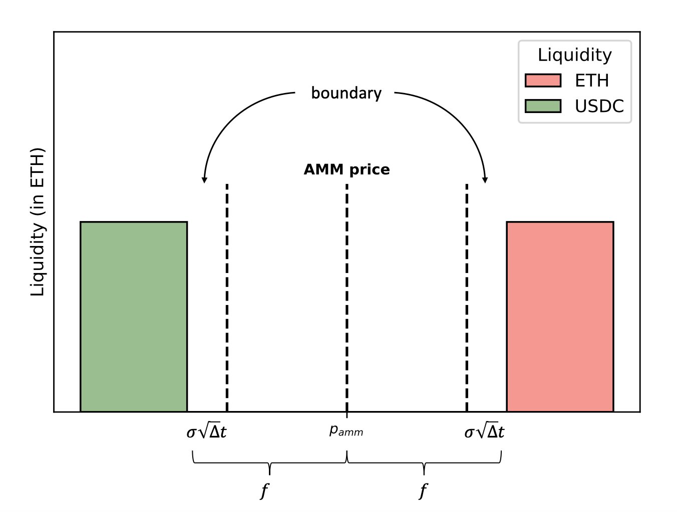
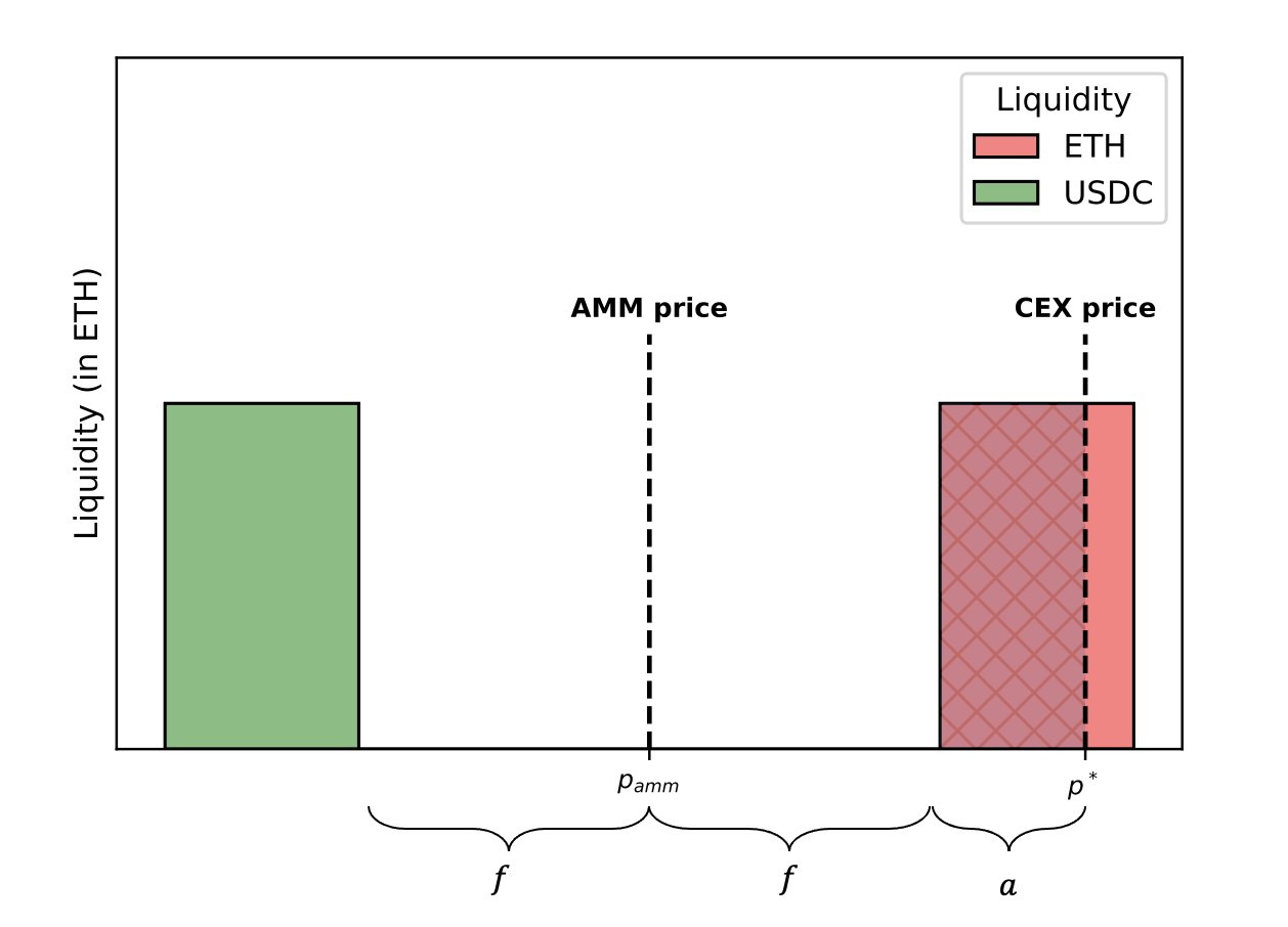
• When the CEX price jumps outside of the AMM’s no-trade region, the arbitrageur trades. At this point, the difference in the CEX price and AMM price net fees is $\sigma \sqrt{\Delta t}$ . The size of the trade is also $\sigma \sqrt{\Delta t}$. Hence profit is $\sigma^{2}\Delta t$.
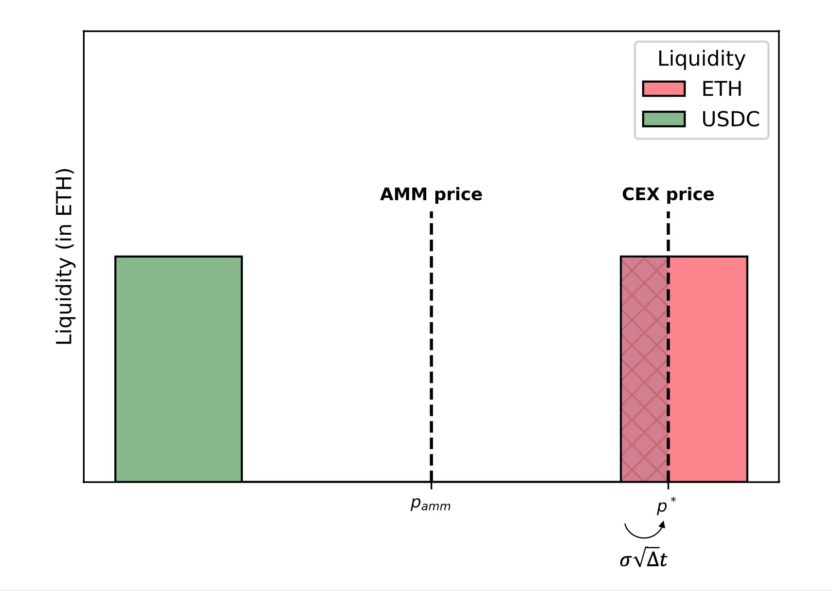
• In what fraction of blocks does the price jump outside the no-trade region? To jump outside, you need to be $\sigma \sqrt{\Delta T}$ or less away from one of the boundaries. The price is uniform inside the no-trade region (see the graph of the mispricing process above), so the probability you jump out is the size of the step divided by half the spread: $\sigma \sqrt{\Delta t}/ {\gamma}$.
• Over a long time $T$, there are $T/\Delta t$ blocks. So, the number of blocks in which there is an arbitrage trade is $(T/\Delta t)\times (\sigma \sqrt{\Delta t}/\gamma) = T \times \sigma /(\gamma \sqrt{\Delta t})$.
• Multiplying the number of blocks with an arbitrage trade by the profit, yields $T \times (\sigma^{3}/\gamma) \times \sqrt{\Delta t}$.

Intuitively, $\overline{\mathsf{ARB}}$’s dependence on $\Delta t$ and $\gamma^{-1}$ makes sense. Theoretical pre-fee arbitrage profit, $\overline{\mathsf{LVR}}$, is independent of block times and fees, as CEX prices are exogenous. But given a certain swap fee, shorter block times lead to more trade volume and more fees paid to LPs. Say the ETH price is 1000 at 9am, slowly rises to 2000 at 9pm, and slowly reverts to 1000 tomorrow at 9am. If arbitrageurs can only trade at 9am, no trades happen. If arbitrageurs can trade every hour, more trades happen and more fees are paid to LPs. Interestingly, you can show less volatile block times also help LPs by generating more trade volume.

Special Cases of $\gamma$ and $\Delta t$

As we noted, the approximations above hold in the small fee, fast block time regime ($\gamma \rightarrow 0$, $\Delta t \rightarrow 0$) and are quite accurate for practical parameter settings. Below we walk through a few special cases.

• If, $\gamma = 0$ and $\Delta t = 0$, then $\overline{\mathsf{ARB}} = \overline{\mathsf{LVR}}$. Recall this case is exactly the setting of the original LVR paper.
• If $\gamma = 0$ and $\Delta t \rightarrow 0$, then $\overline{\mathsf{ARB}} = \overline{\mathsf{LVR}} + o(1)$. The rate of arbitrage profits is constant with respect to block time. It does not scale as $\sqrt{\Delta t}$. When there are no fees, the size of the no-trade region is zero. So, intuitively, arbitrageurs trade every block and extract approximately the same profits independent of the block time.
• If $\gamma > 0$ and $\Delta t = 0$, then $\overline{\mathsf{ARB}} = 0$. We can intuit this result from the small fee, fast block time regime, where we know that $\overline{\mathsf{ARB}} \rightarrow 0$ as $\Delta t \rightarrow 0$. Since the instantaneous rate of profit is 0 in the limit, arbitrageurs would have to trade in infinitely large size to generate profit. So, any non-zero swap fee implies infinite fees. However, the upper bound of profits is LVR, which is finite. Hence, arbitrageurs are unwilling to pay infinite fees for finite profits. For a formal result in this vein, check out Evans, Angeris, Chitra 2021. Another related result is Tassy and White 2020 who study an LP’s expected log wealth in a continuous time setting. Check here for a discussion around the assumptions in the latter paper.

Gas Costs

All the models discussed so far ignore gas. Intuitively, we expect lower gas to have the same effect as fast block times. For a fixed amount of LVR, lower gas should drive more trade volume and fees.

As usual, @0x94305 provides a useful result. In a world with with gas, arbitrageurs do not trade as soon as the CEX price exceeds the AMM price net swap fees. Instead, they need an extra deviation, $a$, to justify the trade. Note that $a$ itself is not the gas cost. Instead, $a = 2\sqrt{\frac{F}{L\sqrt{P}}}$, where $F$ is the gas cost, $L$ is the CPMM’s liquidity and $P$ is the CEX price. Assuming that $a$ is roughly constant over time, we have: $\overline{\mathsf{ARB}} \approx \mathsf{const} \times \sigma^{2} \times \frac{1}{1 + \frac{2\gamma}{a + \sigma \sqrt{2\Delta t}}}$ Say $\sigma \sqrt{2 \Delta t} \ll a$. Then, reducing gas costs by 50\% means that LPs could reduce swap fees by ~30% and face the same losses.

So far, the framework has been that LPs and arbitrageurs are playing a zero-sum game. Gas changes the picture because gas fees paid by arbitrageurs do not go to LPs. So, reducing gas helps both parties: it reduces LP losses and increases realized arbitrageur profits.

AMM Design

Before thinking about AMM design, let’s breakdown LP profitability. The LVR framework completely ignores one side of the picture, fee income earned from non-toxic flow. The full picture looks closer to: $\overline{\mathsf{LP\, PnL}} \approx \overline{\mathsf{FEE}}_{u} - \overline{\mathsf{ARB}}$ where $u$ indicates uninformed. Now, we know what levers we can pull to improve PNL.

Below, we will explore two approaches to LVR mitigation.

1. Making passive LPs more active: The goal here is to mimic professional market makers, who update quotes in response to any information about the fair value of an asset and the toxicity of incoming flow. The hope is to hold constant $\overline{\mathsf{FEE}}_{u}$ and decreasing $\overline{\mathsf{ARB}}$ with dynamic fees, swap-based fee discrimination and oracles.
2. MEV recapture: An alternative line of thinking is to leave the internal mechanics of AMMs largely unchanged, but force informed traders to compensate LPs for the right to arbitrage the pools. Arbitrageurs bid aggressively in the MEV-boost auction to guarantee the right to TOB execution, so block proposers capture a slice of arbitrageur profits. Re-directing that value to LPs instead would improve their profitability. Conceptually, let’s say $\overline{\mathsf{REV}}$, denotes revenue earned from MEV recapture. Then, we have:$\overline{\mathsf{LP\, PnL}} \approx \overline{\mathsf{FEE}}_{u} - \overline{\mathsf{ARB}} + \overline{\mathsf{REV}}$The idea is to make $\overline{\mathsf{REV}}$ close to $\overline{\mathsf{ARB}}$, driving arbitrageur profit margins as small as possible. The primary mechanisms for doing so are auctions, but there is an open question around censorship resistance related to these designs.

Finally, we discuss some improvements specific to concentrated liquidity AMMs and thoughts on how recent developments in the AMM space affect implementing LVR mitigations.

Making Passive LPs More Active

Dynamic Fees

In order book settings, market makers adjust spreads to optimize risk-return. When uncertainty is low, they quote tight spreads to attract volume. When uncertainty is high, they quote wide spreads to manage inventory risk and adverse selection. If a large buy/sell order comes in, they will fade incoming trades by adjusting prices up/down.

How do we approximate such strategies on AMMs? Uniswap v3 supports several fee tiers. In theory, LPs could actively manage liquidity across fee tiers. However, per analysis from the Ambient Finance team LPs do not act optimally. They oversupply to the 0.05% pool, even though the 0.3% pool generates more fee revenue and outperforms in times of high volatility. Although gas to mint/burn positions is part of the picture, LPs behavior is similar on both Ethereum and Polygon. So, dynamic fee policies adjust fees automatically over time on behalf of LPs.

Scaling Fees with Volatility

One strategy is to scale fees with volatility. From the LVR model, we know that $\overline{\mathsf{ARB}} \propto \sigma^{3}/\gamma$, so it keeps arbitrage profits in check. What happens to $\overline{\mathsf{FEE}}_{u}$? For any AMM, the answer will depend on liquidity at other venues and the fee elasticity of uninformed traders. If users get optimally routed via DEX aggregators and there is a competing pool, all non-toxic flow would disappear if we charged even a 1bp premium. If users are sticky, this is less of a problem. The basic intuition here is that in times of high volatility, more fee revenue hopefully compensates LPs for more adverse selection.

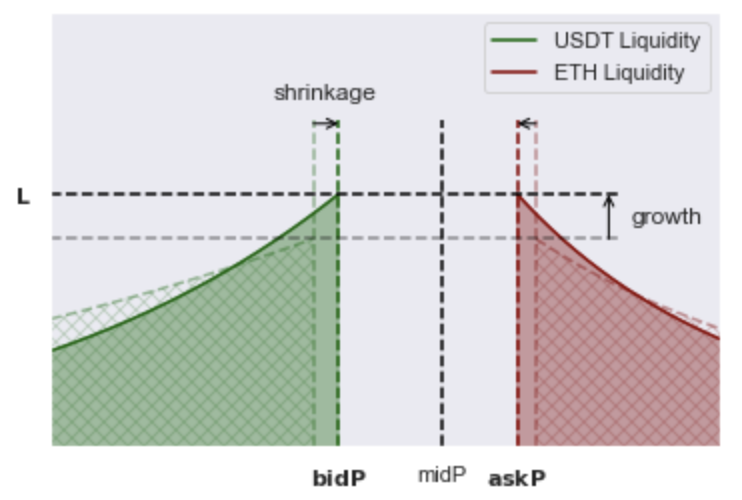
In practice, a few approaches have been explored. Trader Joe and KyberSwap measure volatility from recent volume and price impact in the pool. @0x94305 has previously proposed LTAMM, which can be visualized as a synthetic order book that runs a two-sided Dutch auction for the bid and ask side liquidity. At each block, the spread contracts at a rate (shrinkage) and liquidity concentrates at a rate (growth). When a swap is executed, the spread widens and liquidity flattens. When volume is low, the spread will tend to tighten. When volume is high, the spread will tend to widen.

Statistical Models

As explained above, it is difficult to determine optimal fees without strong assumptions about non-toxic flow. However, it is clear that competing liquidity venues have an important role. If all Uniswap v3 liquidity charges between 0.05% and 1%, then we should not go outside that range. If we go too low, we are unlikely to gain more volume than the 0.05% pool. If we go higher than 1%, we will get essentially no volume.

Based on this insight, the Ambient Finance team explores a statistical approach to dynamic fees. They train a linear model of which predicts which Uniswap fee tier will experience the most fee accrual in the next time period based on the fee accrual, swap volume and volatility of the tiers from the past few time periods. The tier with the highest predicted payoff is selected. The study suggests such a dynamic fee policy could deliver better returns for LPs:

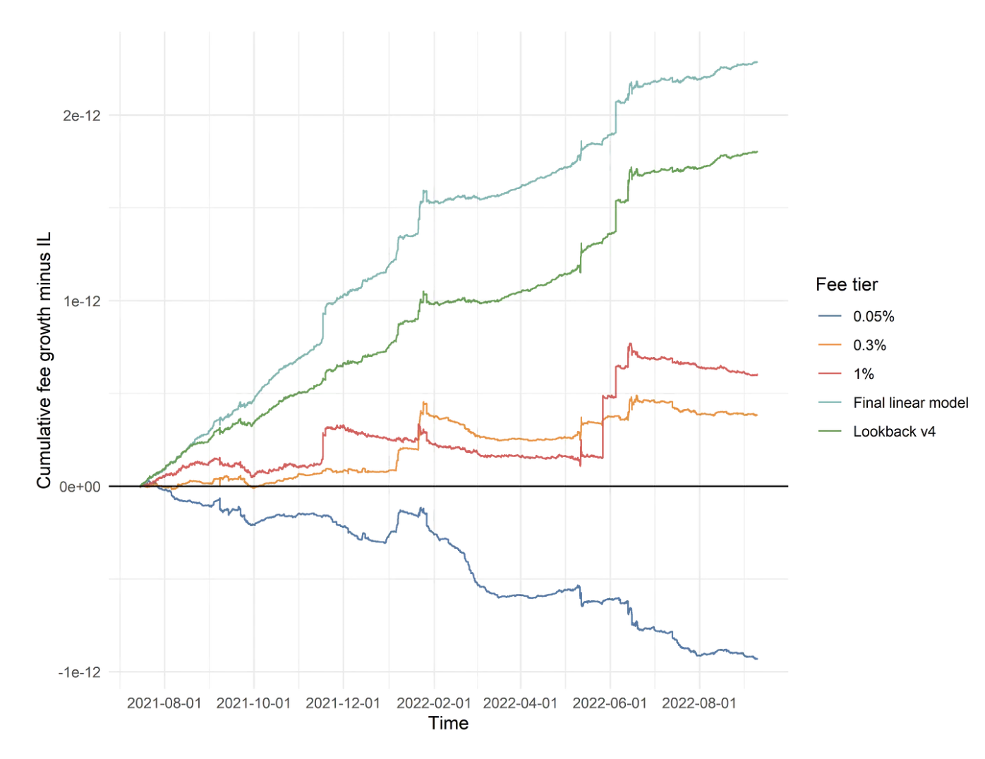
There are caveats about the generalization of a model fitted to Uniswap data. What looks optimal on Uniswap pool is unlikely to be optimal for an AMM with less access to non-toxic flow. However, in general, the strategy holds: AMMs can build statistical models from on-chain data to calibrate dynamic fees.

Asymmetric Spreads

In this thread, @0x94305 suggests a dynamic fee approach that relies on asymmetric fees:

Say in block t, the AMM price went up by Δ. Then, at the top of block t+1, raise the fee for buys and lower the fee for sales by δ=cΔ, for some c>0. Only make sure that neither fee ever gets negative.

As an example, say the ETH price on the CEX jumps and an arbitrageur swaps ETH for USDC on the AMM. Afterwards, a standard AMM quotes a symmetric $2f$ spread with the best ask at the CEX price. The new AMM also quotes a $2f$ spread, but it is asymmetric. 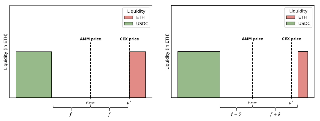With a symmetric spread, just after pushing the AMM’s best ask to the CEX price, any movement in the same direction creates another arbitrage. On the other hand, the CEX price has to cross the $2f$ spread to make arbitrage profitable on the bid side. Hence the direction of toxic flow is autocorrelated, which holds up in the data. We expect the direction of net non-toxic flow is random. So, with an asymmetric spread, we penalize toxic flow more than non-toxic flow. Simulations suggest this could cut LP losses by 10-15%. A conceptually similar approach is currently implemented by Lifinity’s rebalancing mechanism.

Note that this mechanism has a nice property. On average, it charges uninformed traders the same fee and informed traders a higher fee. So, $\overline{\mathsf{FEE}}_{u}$ holds constant and $\overline{\mathsf{ARB}}$ decreases. In the earlier designs, the trade-off between these two terms is less clear.

Swap-Based Fee Discrimination

Dynamic fees are a global mechanism which modify fees over time for all traders. A more granular mechanism is to discriminate between informed and uninformed traders on a swap-by-swap basis and charge high fees on toxic flow and low fees on non-toxic flow.

Fee discrimination is common in TradFi. In fact, it is exactly what motivates PFOF, where market makers like Citadel buy non-toxic flow from retail trading venues like Robinhood and offer competitive spreads on those trades.

Empirical Facts

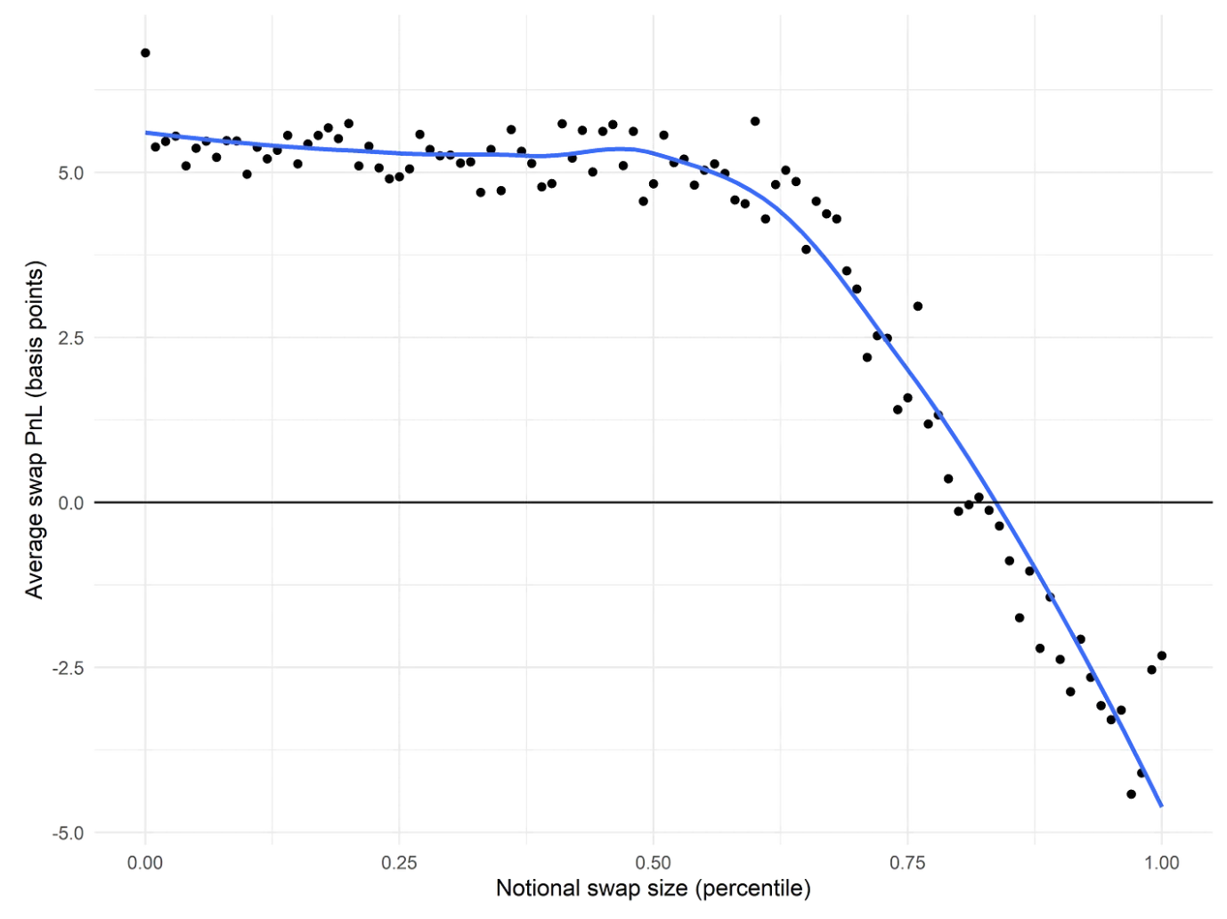
@0xfbifemboy has an excellent series of posts documenting what types of swaps tend to be toxic vs non-toxic empirically. The analysis uses data on ETH/USDC Uniswap v3 pools through Sep 2022. It relies on computing per-swap PnL from 5-minute Binance markouts. The results confirm common intuitions about toxic vs non-toxic flow in crypto. Below is quick summary.

Note that all the following graphs show swap PnL experienced by LPs, not traders. Negative swap PnL means LP losses. Positive swap PnL means LP profits.

• Larger swaps are more toxic.
• Swaps from wallets with more a more extensive swap history are more toxic. However, there is a subset of frequent swappers who are non-toxic, including addresses associated with a CoW Swap order solver and the well-known MEV bot 0xa57. Fresh wallets are always non-toxic, independent of swap size.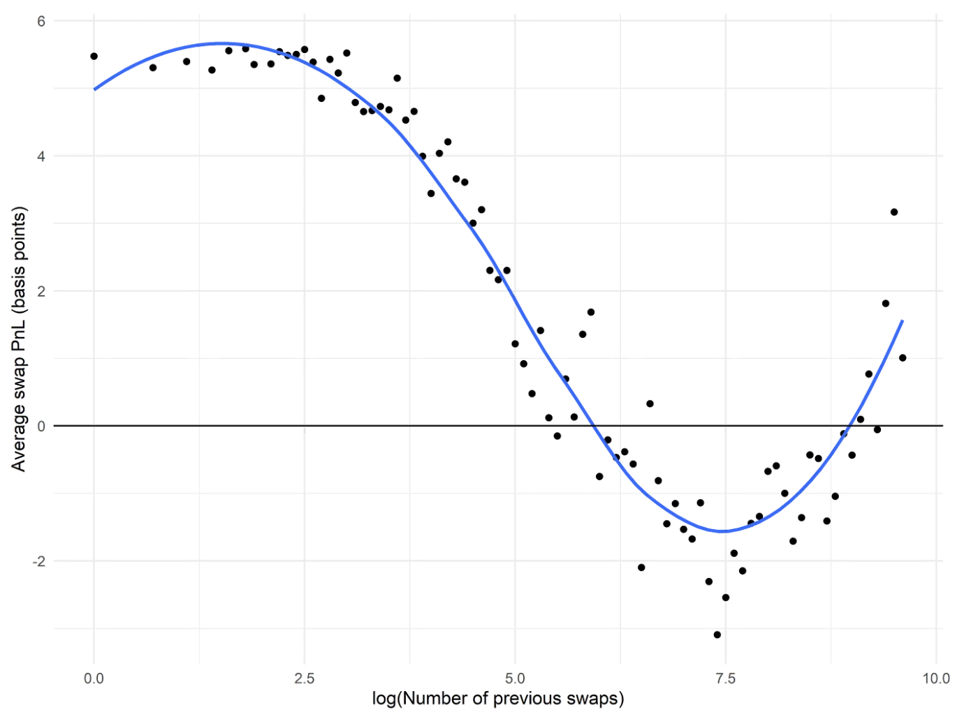
• There is a small group of 364 extremely toxic wallets responsible for generating nearly -$150 million in losses for LPs in the pool. All other wallets generate $104 million in profits for LPs.
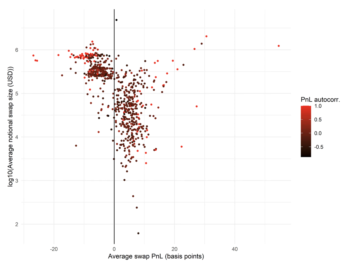
• One can roughly cluster wallets into toxicity levels from the graph below, which shows a wallet’s swap size vs PnL and is colored by the wallet’s swap PnL autocorrelation.
  • High toxicity - Wallets with negative PnL, large swap size and PnL autocorrelation > 0.9.
  • Medium toxicity - Wallets with negative PnL, large swap size and PnL autocorrelation < 0.9.
  • Low toxicity - Everyone else.
• High/medium toxicity wallets swap more frequently and routinely switch swap direction.
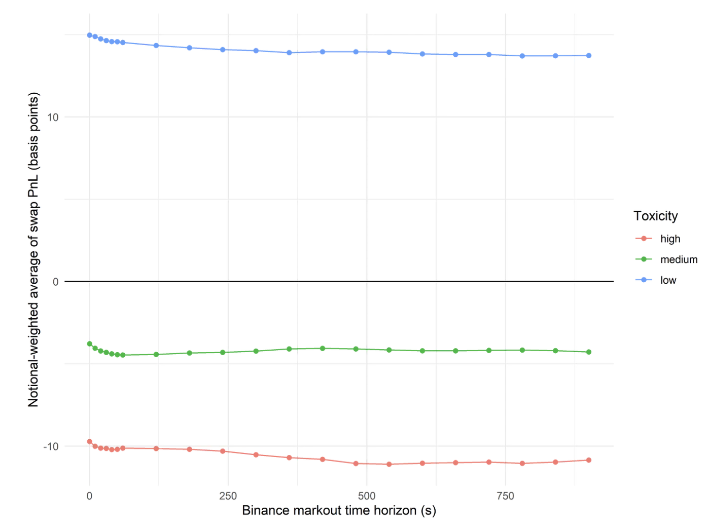
• High/medium toxicity wallets experience significant alpha decay. Specifically, a comparison of swap PnL over different Binance markout durations shows swap PnL plateaus after ~1 minute for these wallets.
• Swaps which interact with the Uniswap v3 router contract, CoW Swap, MetaMask and DEX aggregators are non-toxic. Swaps which originate from MEV contracts are toxic with the exception of atomic arbitrage bots.

Implementation

The results above suggest AMMs should charge higher fees to wallets which execute in size, have an extensive swap history or come from a blacklist of toxic addresses. But informed traders can easily split up swaps and create new EOAs. In general, penalizing toxic flow creates an adversarial game where the AMM and arbitrageur come up with increasingly sophisticated strategies to thwart one another.

However, there are more viable strategies. First, AMMs can incentivize uninformed traders to signal non-toxicity. How exactly?

• Long-term orders: If you specify that a swap can be executed over several blocks, you are probably non-toxic. We know that toxic flow has alpha that decays within ~1 minute and needs fast settlement to capitalize on arbitrage. One solution is TWAMM style long-term orders with fees that decay with expiry time. In general, such a feature should attract non-toxic flow from DAOs and protocols who need to execute large on-chain swaps.
• Venue-based discounts: If your transaction comes from a whitelist of addresses including CoW Swap, MetaMask and DEX aggregators, you are non-toxic. It is infeasible for arbitrageurs to hide in these venues since uncertainty around routing and settlement times eliminates any alpha. Balancer has implemented this approach by approving 50-80% fee discounts for CoW Swap and 1Inch solvers.

Second, @0xdoug points out AMMs can design reputation systems, which encourage actors to cooperate with the AMM on fee discrimination. The Ambient Finance team suggests a relayer approach, which provides a fee discount to privileged actors. These (off-chain) relayers are responsible for sourcing order flow, implementing wallet profiling schemes, and sending non-toxic swaps to the AMM. Periodically, AMM governance evaluates swap PnL from the relayers and removes those who “misbehaved.” Relayers want to stay whitelisted since they earn some of the spread between the standard and discounted AMM fee.

Quoting Closer to Fair Value

We know LVR is driven by price slippage from a AMM executing at prices worse than fair value. If LPs quote closer to the CEX price, they can better replicate the execution of the rebalancing strategy and reduce arbitrage profits. In theory, given access to the CEX price, $P_{t}$, an AMM could simply offer a price of $P_{t} - \epsilon$. This talk by Anthony Lee Zhang more precisely explains how such an AMM would eliminate LVR.

Oracles

The obvious design here is to use a high-frequency oracle of CEX prices as an input to the AMM. On Solana, Lifinity is an AMM that provides liquidity around an oracle price pulled from the Pyth Network . Since Pyth prices are calculated from data collected by market makers and exchanges, it should approximate CEX prices.

When using an oracle there are important considerations to keep in mind:

1. On Ethereum, CEX-DEX arbitrageurs can bid in MEV-boost auctions for TOB execution, getting ahead of any oracle update. To prevent front-running attacks, one could lock the AMM pool until after the update. Such a feature degrades the UX for uninformed traders and reduces the amount of non-toxic flow.
2. There are always questions around oracle accuracy and robustness. For example, the Lifinity team has documented Pyth prices can lag CEXes and, as a result, their pools sometimes underperform a CPMM. Importantly, if an oracle reports a price far away from fair value due to manipulation, LPs will lose more to LVR than otherwise.

MEV Recapture

McAMM

The idea behind McAMM is to move the auction for TOB execution from the consensus layer directly to the AMM’s smart contracts and pass on the auction proceeds to LPs.

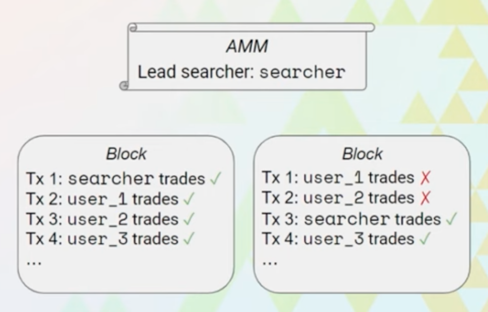
Specifically, McAMM’s router auctions off TOB access to all pools. The winner’s address is stored in a variable leadsearcher. At every block, the pool checks if the leadsearcher has traded. If so, other trades execute afterwards. Otherwise, they revert. Since any fee discount should be priced into auction bids, the leadsearcher pays no fees to enable more efficient arbitrage.

The specifics of the auction mechanism are flexible. A simple design is a Harberger tax-style continuous auction. The winning bid is staked with the router. Every block $x\%$ of the bid is taken as revenue by the AMM. The leadsearcher loses status once the stake is fully depleted, which takes $1/x\%$ blocks. However, at any point, a competitor can take over by bidding $y\%$ more than the current bid. In that case, the previous leadsearcher’s remaining stake is returned. This implementation mimics Eden slot auctions.

For McAMM to work correctly, transactions have to be properly sequenced by block builders. Normal user trades come after leadsearcher trades. It would make sense for builders to respect this ordering since they target blocks with maximum gas consumption to earn priority fees. Placing normal user trades first would cause reverts and less gas consumption.

Optimal Auction Frequency

An important question is what is the optimal auction frequency? In the implementation above, smaller $x$ values correspond to less frequent auctions. The implicit “bid duration” is $1/x\%$ blocks.

Longer bid durations seem to reduce competition. Trading over a longer horizon is easier with access to more capital. Also, some stat arb alphas exist for short periods of time and disappear. Hence smaller CEX-DEX teams running niche strategies may be unsure they can outcompete over long horizons. So, in a world of less frequent auctions, we expect participants will demand larger risk premiums and submit smaller bids, which decreases LP revenue.

Another concern is simply that less frequent auctions imply longer monopolies on leadsearcher status. From the leadsearcher’s perspective, the ability to lock pools by refusing to trade means a longer bid duration is similar to increasing the block time, $\Delta t$, in the LVR model. It will often be profitable to hold off until the last block when CEX prices have had the most time to diverge and execute a single set of trades, paying gas only once. What are the downsides? First, locking the pools deteriorates the UX for normal users. Second, it can create hack risk for other protocols using a stale TWAP oracle from the AMM.

The upside to less frequent auctions is less value leaked in gas costs, which would show up as higher bids and more LP revenue.

Redistribution Mechanism

The best way to re-distribute auction proceeds across LPs is unclear. In the original McAMM proposal there is one global auction for all pools. However, in any block, the amount of LVR experienced by a given LP will depend on the pool and the LP position itself (price range and concentration).

A simple heuristic would be to allocate across pools proportionally to the pool’s price change over the block. Within a given pool, in-range LPs would be compensated proportionally to their liquidity. However, this mechanism is far from perfect since the leadsearcher could create their own tokens, LP into pools for these tokens and execute large trades in order to win back some of the auction proceeds.

Diamond Protocol

McMenamin, Daza & Mazorra 2022 propose the Diamond protocol, an AMM design that relies heavily on block builders to share LVR between LPs and arbitrageurs.

To understand Diamond, it is useful to think of block builders as running CEX-DEX arbitrage. We know that integrated builder-searchers already exist. Even if some builders are not stat arb teams, they still run order flow auctions which capture the value of LVR via inclusion tips from external arbitrageurs.

With this mind, the protocol works as follows.

1. The AMM processes a pool unlock transaction:
   • The block builder must deposit collateral for both tokens, $C_{x}$ and $C_{y}$.
   • If this transaction is not included, all trades revert.
2. Trades are then executed against the pool per the AMM invariant curve:
   • The ordering is up to the block builder, enabling them to capture any value from CEX-DEX arbitrage at the TOB.
   • However, there is an important constraint. Any trade $i$ reverts unless the deposited collateral exceeds the product of a LVR retention parameter $\beta \in [0, 1]$ and the change in reserves from the start of the block: $C_{x} \geq \beta \cdot \left(x_{i} - x_{\mathsf{start}}\right) \quad \text{and} \quad C_{y} \geq \beta \cdot \left(y_{i} - y_{\mathsf{start}}\right)$
3. At the start of the next block, the block builder is refunded and the pool is rebalanced:
   • WLOG say in the last block, the pool sold token $x$ and bought token $y$, so $\Delta x = x_{\mathsf{start}} - x_{\mathsf{end}} > 0$ and $\Delta y = y_{\mathsf{end}} - y_{\mathsf{start}} > 0$.
   • $\beta \cdot \Delta y$ tokens are removed from the pool and sent to the block builder. All of $C_{y}$ is refunded.
   • $\beta \cdot \Delta x$ tokens are taken out of $C_{x}$ and added back to the pool. The rest of $C_{x}$ is refunded.
   • After these transfers, the pool price is different from the pool price at the end of the block. Specifically, we have $\frac{y_{\mathsf{start}} + (1 - \beta) \cdot \Delta y}{x_{\mathsf{start}} - (1 - \beta) \cdot \Delta x} < \frac{y_{\mathsf{end}}}{x_{\mathsf{end}}}$.
   • To fix the price, an additional $\Delta x_{\mathsf{vault}}$ is removed from pool such that $\frac{y_{\mathsf{start}} + (1 - \beta) \cdot \Delta y}{x_{\mathsf{start}} - (1 - \beta) \cdot \Delta x - \Delta x_{\mathsf{vault}}} = \frac{y_{\mathsf{end}}}{x_{\mathsf{end}}}$. These tokens added to a separate vault contract.
4. A periodic auction is run to convert vault tokens and re-add them to the pool:
   • Say the vault currently has tokens, $x_{\mathsf{vault}}$ and $y_{\mathsf{vault}}$.
   • Half of each of the reserves are auctioned off in return for the other asset in the pair. Let the auction proceeds be $y_{\mathsf{bid}}$ and $x_{\mathsf{bid}}$, respectively.
   • The remaining reserves and auction proceeds, $(x_{\mathsf{vault}}/2) + x_{\mathsf{bid}}$ and $(y_{\mathsf{vault}}/2) + y_{\mathsf{bid}}$, are transferred out of the vault back the the pool.

Let’s figure out why the protocol works. Given all the transfers to and from the block builder, we see the AMM sells a total of $(1 - \beta) \cdot \Delta x$ tokens and buys a total of $(1 - \beta) \cdot \Delta y$ tokens. However, the pool price still equals the price in a world where the full swap of $\Delta x$ for $\Delta y$ is executed. So, the AMM has aligned the pool and CEX prices, while retaining a $\beta$ fraction of the LVR. The retained LVR effectively comes from the tax imposed on the builder’s collateral and gets transferred to the vault. The AMM can then sell vault tokens and add liquidity back. The key assumption here is that the conversion auction is competitive, so vault tokens are sold at close to CEX prices. Otherwise, the LVR situation for LPs is no different from an AMM executing the full swap below fair value.

Setting the LVR Retention Parameter

For the Diamond protocol to function, the LVR retention parameter needs to be optimized. Setting $\beta$ closer to 1, is better for LPs since they retain more LVR, ensuring $\overline{\mathsf{REV}} \approx \overline{\mathsf{ARB}}$. However, if set too high, block builders will be unwilling to unlock the pool and process trades as their profits margins are small. A simple idea is to make $\beta(\cdot)$ a decreasing function and pass in the number of blocks since the last swap, which essentially makes Diamond protocol a Dutch auction for the LVR that can be extracted from the pool. With sufficient competition among block builders, LPs should recapture maximum MEV.

Censorship Resistance

In theory, competition among CEX-DEX arbitrageurs should drive up bids in the McAMM and Diamond protocol auctions such that $\overline{\mathsf{REV}} \approx \overline{\mathsf{ARB}}$. However, this assumes honest block proposers who ultimately determine which transactions get included. An arbitrageur seeking to win an auction with an uncompetitive bid can bribe the proposer to censor other bids. In this case, arbitrageurs and proposers keep most of the LVR instead of passing it on to LPs and we end up with $\overline{\mathsf{REV}} \ll \overline{\mathsf{ARB}}$. In McAMM, arbitrageurs can simply exclude other bids to take on the role leadsearcher for cheap. In the Diamond protocol, a similar problem exists for the vault conversion auctions. In all cases, value that LPs expect to earn via MEV recapture is leaked at the consensus layer, similar to the status quo.

Fox, Pai, & Resnick 2023 study censorship resistance in on-chain auctions formally. The authors model a smart contract selling a good via a second-price, sealed-bid auction. Users submit private bids to the auction as transactions (e.g. using a commit-reveal scheme) and public inclusion tips to block proposers. Despite the private bids, users learn about bids from the public tips. For example, if your tip is $t$, it is clear that you value the good as $v \leq t$ and would bid no more than $v$. After seeing the tips, a user can bribe the proposer to censor bids if it would be profitable to do so. The resulting equilibrium is the colluding user wins the auction with high probability and large surplus, driving down auction revenues earned by the seller.

Off-chain Auctions

One solution to censorship resistance is to bypass the public mempool all together and run auctions off-chain through a trusted third-party operator. The operator honestly collects bids from all participants, determines the winner, and executes relevant transactions. For example, in McAMM, the operator signs a message giving the winner leadsearcher role and sends a transaction transferring auction proceeds to the router. Of course, the downside is sacrificing maximum decentralization.

MCBP

An alternative solution suggested in Fox, Pai, & Resnick 2023 is multiple concurrent block proposers (MCBP). The idea is that weak censorship resistance in blockchains results from single proposer monopolies on transaction inclusion.

In MCBP, there are $k$ concurrent proposers and transactions included by at least one of the proposers is included on-chain. Tips take a two-dimensional form $(t, T)$ where $t \ll T$. If a single proposer includes the transaction, they are paid $T$. If multiple proposers include the transaction, they are each paid $t$. This conditional tipping logic sets up a prisoner’s dilemma-type scenario. The dominant strategy for each proposer is to include the transaction. See the payoffs below for the $k = 2$ case from Mallesh Pai’s talk: Hence the cost of inclusion is $kt$. On the other hand, an arbitrageur has to pay each proposer $T$ in order to censor the transaction for a total cost of $kT$. Given that $kT \gg kt$, in the resulting equilibrium, the probability the arbitrageur bribes is zero and all auction bids get included on-chain.

Of course, MCBP would require consensus-layer modifications to Ethereum. However, it is an option for appchain AMMs. Duality Labs has announced they are building Multiplicity, a modification to the Tendermint protocol that allows non-leader nodes to include transactions in a block. The goal is to enable competitive on-chain MEV auctions for their Cosmos-based DEX.

Ex-Ante vs Ex-Post Auctions

McAMM runs an ex-ante LVR auction, while the Diamond protocol runs an ex-post LVR auction. In an ex-ante auction, arbitrageurs bid ahead of time based on the predicted LVR over the next few blocks. In an ex-post auction, arbitrageurs can explicitly calculate the value from CEX-DEX arbitrage over the course of a slot and pay a $\beta(\cdot)$ fraction of this realized LVR to LPs. An ex-post auction is closer to how things currently work in MEV-boost, where stat arb teams update bids over the course of the slot.

There are trade-offs to consider here. An ex-ante auction may be less competitive because it disadvantages risk-averse arbitrageurs, who are unwilling to absorb uncertainty around the amount of extracted LVR. However, it is also better suited for running on-chain. An ex-post auction has to run every block. In an ex-ante auction, leadsearcher’s maintain status for a while, so the auction can run over multiple blocks. A multi-block auction is a bit more censorship resistant because it requires the colluding user to bribe several proposers, which is relatively expensive. Managing censorship in an ex-post auction without MCBP likely requires moving it off-chain. This is effectively what is going on with the Diamond protocol, which assumes builder competition through the off-chain, MEV-boost auction to maximize the LVR retention parameter $\beta$.

Making Passive LPs More Active vs MEV Recapture

For an excellent comparison of the two LVR mitigation approaches above, check out the following Twitter spaces discussion.

There are two clear downsides to strategies that make LPs more active. First, they may do more harm than good. A simple example is a manipulated oracle, which posts a price further away from fair value than the AMM’s original pool price. Ideally, new AMM features should be constrained to guarantee LPs an upper bound on $\overline{\mathsf{ARB}}$, no larger than the CPMM case. Second, there is a risk of overfitting to historical data. For example, parameters in a dynamic fee model will quickly become outdated as arbitrageurs adapt their behavior to maximize profit.

MEV recapture mechanisms avoid these issues. Given there is no change to the internal AMM mechanics, LVR can be no worse than the status quo. $\overline{\mathsf{ARB}}$ remains the same and $\overline{\mathsf{REV}}$ is guaranteed to be non-negative. Further, they require no fine-tuning. The decision of how to value LVR is passed on to professional stat arb teams, who automatically reflect any new information into their auction bids. One concern is that auctions may be uncompetitive since there are barriers to entering the CEX-DEX arbitrage business. Stat arb teams need large amounts of on-chain capital, low-latency infrastructure to connect to CEXes and MEV-boost relays, and expertise in managing inventory risk. If a small number of players dominate, they may hold onto large profit margins. Recall the Frontier Research study estimated 37-77% of profits are paid to proposers, so that is likely an upper bound on what can be recaptured by LPs.

Note that both approaches could likely be combined in a clever AMM design.

LVR Mitigation for Concentrated Liquidity AMMs

Eliminating JIT Liquidity

JIT liquidity has a negative effect on passive LP profitability. First, JITers directly dilute fee revenue. Second, they expose LPs to relatively more toxic flow. JITers hedge off-chain and actively track CEX prices. Hence they will tend to only fill swaps which move the AMM away from the CEX price. Arbitrageur swaps which move the AMM towards the CEX price will get offloaded on to passive LPs. Only 0.3% of all liquidity demand on Uniswap is JITed, but this number could grow on high performance chains, where gas costs to mint/burn LP positions are negligible.

An important caveat is that the argument above assumes trader behavior is fixed. Since JITed transactions incur less price impact, large traders may look elsewhere to execute if the JIT-driven price improvement disappears on AMMs. Although @0x94305 shows there are now arbitrageurs who combine sandwiches with JITs, leaving both LPs and traders worse off.

How can AMMs eliminate JIT liquidity? One approach is to impose burn delays. In Ambient, a pool has a minimum time-to-live (TTL) parameter. Each LP position gets timestamped at mint and cannot be burned until the TTL interval has passed. The interval can last anywhere from 0 to 255 seconds. Any TTL > 0 makes atomic JIT infeasible. However, to eliminate JITers willing to hold on to risk for some time, longer TTLs may be necessary. Ambient is flexible in their approach to JIT, allowing governance to atomically and temporarily lower TTL to zero for whitelisted addresses. The thinking is that some JITers will make long-term commitments ensuring low toxicity and market quality.

A second approach is withdrawal fees. Kyberswap effectively uses a vesting schedule for LP fees, so the amount of fees an LP positions earns is proportional to how long it was active. JIT positions are minted/burned quickly, so they are entitled to only a very small fee share.

Automated LP Vaults

Automated LP vaults (Mellow Finance, Gamma Strategies, Kamino Finance, Maverick) have become popular way to help passive LPs manage positions in concentrated liquidity AMMs. Generally speaking, vaults rebalance LP positions around the current/predicted pool price to earn more fees and widen ranges in times of high volatility to reduce LVR.

Given that some LPs are in fact profitable, these vaults could theoretically generate positive returns with properly optimized strategies. In practice, backtests show vault strategies fail to deliver. However, new AMM functionalities which allow LPs to specify dynamic fees or cheaply mint/burn positions may expand the set of viable vault strategies for incremental improvements to LP profitability.

Implementing LVR Mitigation Mechanisms

All of the LVR mitigation strategies discussed above can be implemented from scratch in new AMMs. However, faster experimentation is possible by plugging into Uniswap’s v4 protocol via hooks. The major benefit is that new mitigations can be tested and analyzed without being getting embedded into core AMM smart contracts. Some initial ideas include McAMM-style MEV recapture and volatility-based dynamic fees. A variant of the Diamond protocol using hooks is detailed in the following post. Ambient Finance permission oracles enable similar functionality. Fee discrimination policies can be implemented by providing discounts on certain swaps.

UniswapX also has some important implications. It should lower the barriers to entry for new LVR mitigations, as new pools can receive flow as soon as they integrate with a single filler. On the other hand, UniswapX also introduces an RFQ system which allows a permissioned set of market makers to process orders before they are sent to fillers. As @0xshittrader points out, this dynamic negatively affects LPs since they will receive the same amount of toxic flow, but less non-toxic flow.

Another detail we ignored is the computational complexity of some dynamic fee and fee discrimination mechanisms. In general, it would be infeasible to run a statistical model inside an EVM smart contract. @0xdoug points out that using co-processors may be a solution. AMMs could outsource complex logic to off-chain systems and rely on ZK (e.g. Axiom), TEEs or optimistic proofs to verify the results on-chain.