KDS 2022 - Towards a Theory of Maximal Extractable Value I, CFMMs

A summary of results in this paper by Kulkarni, Diamandis & Chitra, which analyzes MEV in CFMMs.

1. Summary

The goal of the paper is to characterize the maximum value a MEV searcher using sandwich attacks can extract. Key results:

• Reordering MEV: Given order flow of $n$ user trades on a single CFMM, how much can reordering the trades affect excess price impact due to sandwich attacks? The ratio of the price impact of the worst case attack to average case attack is $\mathcal{O}(\log{n})$.
• Routing MEV: Given a network of CFMMs, how much do sandwich attackers affect the routing of trades? Network routing quality, measured by trade-weighted price impact, does not change much, asymptotically. The price of anarchy is $\mathcal{O}(1)$, given sufficient liquidity.

Implicitly, many of these results have a connection to the privacy-utility tradeoff in CFMMs since searcher MEV profit can be mapped to a loss of user privacy.

2. Set-up and Definitions

2.1 Uniswap

We have reserves $R_A$ of token $A$ and reserves $R_B$ of token $B$ with token $B$ as the numeraire. A user’s trade of $\Delta$ units of token $B$ for token $A$ is given by:

$(R_A - \Delta')(R_B + \gamma \Delta) = R_A R_B$

where $1 - \gamma$ is the pool percentage fee and $\Delta'$ is implicitly defined by this equality. The marginal price for a trade of size is $\Delta$ is $p_{AB}(\Delta, R_A, R_B) = \frac{R_A - \Delta'}{R_B + \gamma \Delta}$. The output number of tokens the user receives can be written in terms of the marginal price as:

$G(\Delta) = \frac{1}{\gamma}\left(\frac{-R_A R_B}{R_A + \Delta} + R_B\right)$

Assume that $\gamma = 1$, so that $k = R_AR_B$ remains constant.

2.2 Slippage Limits

Since a user does not know the exact initial price at which their trade executes (other trades may execute first), they specify a slippage parameter $\eta \in [0, 1]$. This Uniswap contract guarantees the user will receive no less than $1 - \eta$ of the amount they would receive in the absence of other trades.

For example, consider a user who submits an trade of size $\Delta_1$ and someone else submits a trade of size $\Delta_2$. A miner cannot execute a sequence of trades $\Delta_2, \Delta_1$ unless:

$G(\Delta_1 + \Delta_2) - G(\Delta_2) \geq (1 - \eta)G(\Delta_1)$

A user is responsible for setting $\eta$, and so submits the trade pair $(\Delta, \eta)$. If the user sets $\Delta$ too high, then it is possible this is a strict inequality. So, an MEV searcher can submit the trade $\Delta_2 = \Delta^{\text{sand}}$ such that: $G(\Delta_1 + \Delta^{\text{sand}}) - G(\Delta^{\text{sand}}) = (1 - \eta) G(\Delta_1)$

The searcher worsens execution for the user by using up any slack in the user’s slippage parameter. The searcher can follow $\Delta_1$ with another trade $\Delta^{\text{sand}'}$ and profit. The triple $(\Delta^{\text{sand}}, (\Delta_1, \eta), \Delta^{\text{sand}'})$ is a sandwich attack. Combining the above equations, one can show that the MEV trade size $\Delta^{\text{sand}}$ is an increasing function of $\eta$ and 0 when $\eta = 0$.

2.3 CFMMs

The above set-up can be generalized to arbitrary CFMMs. A CFMM has reserves $R, R' \geq 0$ and a trading function $\Phi: \mathbb{R}^{2} \times \mathbb{R}^{2} \rightarrow \mathbb{R}$. For any valid trade $(\Delta, \Delta')$, the CFMM satisfies:

$\phi(R, R', \Delta, \Delta') = \phi(R, R', 0, 0)$

Here $\Delta > 0$ (positive sized trade) means the user wants to receive the asset $\Delta < 0$ means the user wants to send the asset to the contract.

For any positive-sized trade $\Delta$, the marginal price is:

$g(\Delta) = \frac{\partial_{\Delta} \phi(R, R', \Delta, \Delta')}{\partial_{\Delta'} \phi(R, R', \Delta, \Delta')}$

The function $g$ is called the price impact function.

A CFMM is symmetrically $\alpha''$-stable if it satisfies:

$|g(\Delta) - g(0)| \leq \alpha'' \Delta$

for $\Delta \in [-M, M]$ and is symmetrically $\beta''$-liquid if it satisfies:

$|g(\Delta) - g(0)| \geq \beta'' \Delta$

for $\Delta \in [-K, K]$. Both $M$ and $K$ are positive constants. Intuitively, this says the for bounded trade sizes, there is a linear upper bound on the price impact of buys and a linear lower bound on the price impact of sells.

Finally, one can show $\Delta' = \int_{0}^{-\Delta} g(t) dt$. The forward exchange function is given by $G(\Delta) = \Delta'$, the amount of output token received for an input of $\Delta$.

3. Sandwich Attacks

The mechanics of the sandwich attack works as follows:

• Searcher seeing the user trade $\Delta$ in the mempool, submits the trade $\Delta^{\text{sand}}$ which satisfies

$G(\Delta + \Delta^{\text{sand}}) - G(\Delta^{\text{sand}})= (1 - \eta)G(\Delta)$

• User trade $\Delta$ goes through
• Searcher recoups initial investment $\Delta^{\text{sand}}$ by submitting trade $\Delta^{\text{sand}'}$. Assuming the searcher is risk neutral, they sell back all the $G(\Delta^{\text{sand}})$ output tokens they hold. We can convert $G(\Delta^{\text{sand}})$ back to units of the input token by implicitly solving the equation.

Keeping track of reserves over the course of these trades, we can see the final PNL in units of the input token is given by:

$\begin{aligned} \text{PNL}(\Delta, \eta) &= \Delta^{\text{sand}'} - \Delta^{\text{sand}}\\ &= \Delta - G^{-1}(G(\Delta + \Delta^{\text{sand}}) - G(\Delta^{\text{sand}}))\\ &= \Delta - G^{-1}((1 - \eta)G(\Delta)) \end{aligned}$

Intuitively, this makes sense. The user trades $\Delta$ input tokens, but only gets back value worth $G^{-1}((1 - \eta)G(\Delta))$ input tokens. The searcher’s PNL is the difference. Notice if $\eta = 0$, then PNL is 0.

3.1 Bounds on Sandwich Attack Profitability

Assumptions:

• $G$ meets a $(\mu, \kappa)$ smoothness conditions. There exist constants $\mu, \kappa$, such that for all $\Delta \in [0, M]$:

$\kappa \Delta \leq G(\Delta) - G(0) \leq \mu \Delta$

• The price impact function $g(\Delta)$ grows sufficiently fast, ruling out constant sum market makers, for example where there is no price slippage.

Under these assumptions, it is possible to derive upper/lower bounds for $\Delta^{\text{sand}'}$, $\Delta^{\text{sand}}$ which depend on the liquidity, curvature and slippage factors. Combining these bounds with PNL formula, leads to the following result.

Result: Let $\gamma = 1 + \Theta(\sqrt{1 + \eta})$. Then, for sufficiently large $\eta$:

$\text{PNL}(\Delta, \eta) \leq C_1 \sqrt{1 + \eta} - C_2 \gamma$

This implies that price impact and searcher PNL is linear in $\gamma$. It grows approximately at a $\sqrt{1 + \eta}$ rate.

3.2 Locality of Sandwich Profitability

Definition: Sandwich attacks for a sequence of trades $\{(\Delta_1, \eta_1), \dots, (\Delta_n, \eta_n)\}$ are strongly local if for any ordered set $(i_1, \dots, i_j)$ where $i_j = n$ and $i_1 \geq 1$, we have:

$\text{PNL}(\Delta_1 + \dots + \Delta_{i_1}) + \dots + \text{PNL}(\Delta_{i_{j - 1} + 1} + \dots + \Delta_{i_j}) \leq \sum_{i = 1}^n \text{PNL}(\Delta_i)$

Strong locality says that it cannot be more profitable to sandwich bundles of trades versus bundling each trade individually. In this case, the problem simplifies since the searcher does not have to solve the Knapsack problem to find the most profitable subset of trades $\Delta_{[1]}, \dots, \Delta_{[k]}$ given blockspace limits.

4. Reordering MEV

Say there are a sequence of trades $T_n = \{(\Delta_1, \eta_1), \dots, (\Delta_n, \eta_n)\}$ with default order $1, 2, \dots, n$. Further, we have a block size $h$ where $3n < h$ (allowing the sandwicher to insert trades). Assume that $\eta_i \leq \eta$ for all $i \in [n]$.

The goal is to analyze, the cost of feudalism (CoF), which captures how much worse a user’s trade execution can be due to a permutation $\pi \in S_n$ of the default trade order.

Definition: CoF is defined as:

$\text{CoF}(T_n) = \frac{\mathbb{E}_{\pi \sim S_n}[\max_{i \in [n]} |\text{PNL}_{\pi(i)}(T_n) - \text{PNL}_{i}(T_n)]|}{\mathbb{E}_{\pi \sim S_n}[\frac{1}{n} \sum_{i = 1}^n |\text{PNL}_{\pi(i)}(T_n) - \text{PNL}_{i}(T_n)|]}$

The numerator describes the expected profit to MEV/miners from sandwiching the worse affected user, over all re-orderings of the trades. The denominator is for the average user.

The following result relies on the smoothness/curvature assumptions from the previous sections as well as the strong locality.

Result: If $T_n = \{(\Delta_1, \eta_1), \dots (\Delta_n, \eta_n)\}$ is strongly local, then $\text{CoF}(T_n) = \mathcal{O}(\log{n})$.

The proof relies on upper bounding the numerator as $\mathcal{O}(\log{n})$ and the denominator as $\mathcal{\Theta}(1)$. The result is fairly positive result on the impact of MEV as blockchains scale/grow, since it shows execution for the worst-case user only grows very slowly, logarithmically, in $n$.

5. Routing MEV

Routing MEV for sandwich attacks describes excess value that sandwichers can extract from user trades over a full network of CFMMs. Here there is a concept of equilibrium routing, in which a user’s trade is routed from source to destination token in a CFMM network such that the price over all paths is equal. The excess price impact of sandwich attacks is the the social cost incurred by the network.

Two illustrative examples:

5.1 CFMM Pigou Example

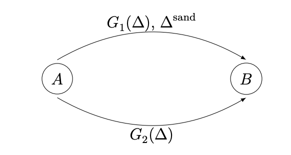
Say there are two Uniswap pools in the CFMM network that trade the same pair of assets, $A$ and $B$. The initial reserves are equal $(R_1, R_1') = (R_2, R_2')$.

In equilbrium, a user who wants to trade $\Delta$ units of $A$ for $B$, will split the trade such that the price over both paths is equal. For the price impact function $g_1$ and $g_2$, we will have $g_1(\alpha^{\ast} \Delta) = g_2((1 - \alpha^{\ast})\Delta)$ where $\alpha^{\ast} \in [0, 1]$, is the fraction of trades made in pool 1. Specifically, $\alpha^{\ast}$ is the solution to:

$\alpha^{\ast} = \text{arg} \max_{\alpha \in [0, 1]} F(\alpha) = \text{arg} \max_{\alpha \in [0, 1]} G_1(\alpha\Delta) + G_2((1 - \alpha)\Delta)$

Note that $F$ ends up being concave, so solving $\frac{\partial F(\alpha)}{\partial \alpha} = 0$, gives the equalibrium condition. In the equal reserves case, this works out to $\alpha^{\ast} = \frac{1}{2}$.

Now if there is a sandwich attacker on pool 1 and the user submits a slippage parameter $\eta$. The optimum changes to:

$\begin{aligned} \alpha^{\ast}(\eta) &= \text{arg} \max_{\alpha \in [0, 1]} F(\alpha, \eta)\\ &= \text{arg} \max_{\alpha \in [0, 1]} G_1(\alpha\Delta + \Delta^{\text{sand}}_{\alpha, \eta}) - G_1(\Delta^{\text{sand}}_{\alpha, \eta}) + G_2((1 - \alpha)\Delta) \end{aligned}$

This comes from directly using the optimal MEV sandwich equation. As expected, for $\eta > 0$, the equilbrium $\alpha^{\ast} < \frac{1}{2}$. The user moves away from pool 1, since the sandwicher makes it more expensive to trade there. The larger the $\eta$, the closer $\alpha^{\ast}$ is to 0 and the smaller the optimum $F(\alpha^{\ast}, \eta)$.

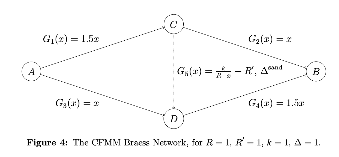
5.2 CFMM Braess Example

A somewhat counterintutive example here shows that the presence of sandwich attacks improves network flow and the MEV profit is bounded. So, while a single user may experience worse execution, the aggregate social welfare improves.

Three cases:

1. Case 1: There is no CFMM for the pair $C, D$, so $G_{5}(x) = 0$. Since both paths, $A \rightarrow C \rightarrow B$ and $A \rightarrow D \rightarrow B$, cost the same, the fraction of a trade $\Delta$ allocated to both is $(\alpha^{\ast}_1, \alpha^{\ast}_2) = (\frac{1}{2}, \frac{1}{2})$. The net output of token $B$ is:

$G_{\text{case 1}}(\alpha^{\ast}, \Delta) = G_2(G_1(\alpha^{\ast} \Delta)) + G_4(G_3((1 - \alpha^{\ast}) \Delta))$

1. Case 2: There is now a CFMM for the pair $C, D$, so $G_{5}(x) > 0$. Using a symmetry of the price paths, you can get to the output formula below and the equilibrium $(\alpha^{\ast}_1, \alpha^{\ast}_2, \alpha^{\ast}_3) = (0.29, 0.41, 0.29)$. Interestingly, you see that the user’s net output reduces in this case:

$\begin{aligned} G_{\text{case 2}}(\alpha^{\ast}, \Delta) &= G_2(G_1(\alpha^{\ast} \Delta)) + G_5(G_4(G_1(1 - 2\alpha))) + +G_4(G_3(\alpha_2 \Delta))\\ G_{\text{case 2}}(\alpha^{\ast}, \Delta) &< G_{\text{case 1}}(\alpha^{\ast}, \Delta) \end{aligned}$

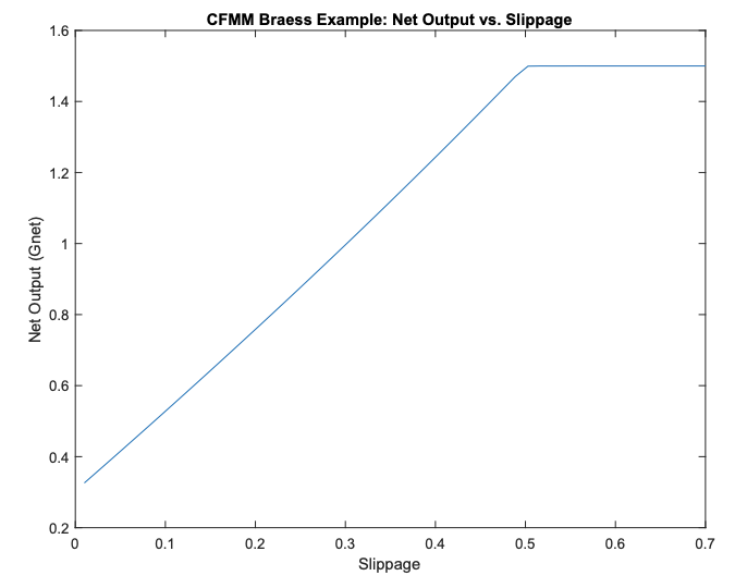
1. Case 3: Add a sandwicher on the $C \rightarrow D$ path and the user now adds a slippage limit $\eta$ for the path $A \rightarrow C \rightarrow D \rightarrow B$. Again, the equilbrium, $\alpha^{\ast}(\eta)$ shifts much like the CFMM Pigou Example and depends on $\eta$. But, here we actually see that as $\eta$ increases, the user moves away from taking the middle path and increases output. This continues the equilibrium converges to case 1, $(\alpha^{\ast}_1, \alpha^{\ast}_2, \alpha^{\ast}_3) = (\frac{1}{2}, 0, \frac{1}{2})$. The presence of the sandwicher forces users to effectively re-allocate across the network to avoid congestion.

5.3 Price of Anarchy

5.3.1 Network Set-up

The theoretical results depend on the following set-up: There is a graph $G = (V, E)$ where each vertex $A \in V$ is a token and each edge $e \in E$ is a CFMM for a pair of assets. For each edge there is an associated price and forward exchange function, $g_{e}(\cdot)$ and $G_{e}(\cdot)$. Each trade is specified as $T = (\Delta_{AB}, \eta_{AB})$ for a trade of $\Delta$ from vertex $A$ to $B$ with a slippage parameter of $\eta$.

5.3.2 Equilibrium Splitting

For a trade $T$, denote the set of all paths from $A$ to $B$ as $\mathcal{P}$. Let $\alpha \in \{\mathbb{R}^{\|\mathcal{P}\|} \: \sum_i x_i = 1\} = S_{\|\mathcal{P}\|}$ be the splitting vector that denotes the fraction of $\Delta$ routed over all the possible paths.

Definition: A splitting vector $\alpha^{\ast} \in S_{\|\mathcal{P}\|}$ is an equilibrium splitting in price, if for all $p \in \mathcal{P}$, when $\alpha_p^{\ast} > 0$, we have:

$g_{p}(\alpha^{\ast}_p) \leq g_{p'}(\alpha^{\ast}_{p'})$

for all other $p' \in \mathcal{P}$.

The implication here is that for all paths on which there is non-zero traffic in equilibrium, the user must face the same price. This is analagous to the equilbrium from the CFMM Pigou Example.

5.3.3 Sandwich Attacks

Much like the for the proof of the PNL bounds for the sandwich attacks, it is possible to upper/lower bound the searcher’s trade size $\Delta_e^{\text{sand}}$ for each edge in the network in terms of the cumulative trade through $e$, $\Delta_e$. It is a bit more complicated here because the user only provides a single slippage parameter $\eta_{\text{AB}}$, so the searcher has to back out the implied slippage $\eta_{1}, \dots, \eta_{\|p\|}$ for each individual edge in a path $p = (e_1, \dots, e_{\|p\|}) \in \mathcal{P}$.

5.3.4 Social Cost and Price of Anarchy (PoA)

To define the social cost, we first define the cost of each edge $e$ in terms of the sandwich size $\Delta^{\text{sand}}_{e}$. The cost for a given edge $e$ is:

$c_{e}(\alpha, \Delta) = p_e(g_e(\Delta^{\text{sand}}_{e} + \Delta_e) - g_e(\Delta_e))$

where $p_e$ is the price of the output token for edge $e$ in terms of the infinitely liquid numeraire, like USD. Here, $c_e$ represents the excess price impact due to the sandwich attack in units of USD per input token.

Definition: The aggregate cost of sandwiching on the network is given by a trade-weighted average:

$C(\alpha, \Delta) = \sum_{e} c_{e}(\alpha, \Delta) \Delta_e$

Definition: PoA is defined as following. Let $\alpha^{\ast} \in S_{\|p\|}$ be any equilbrium splitting. Then:

$\text{PoA}(\Delta) = \frac{C(\alpha^{\ast}, \Delta)}{\inf_{\alpha} C(\alpha, \Delta)}$

This reflects the ratio of the equilbrium social cost to the minimizer.

The final result of the paper shows the $PoA$ is upper bounded by a constant, that depends on the curvature/slippage parameters of the network.

Result: There exists a function $C(\Gamma)$ that is constant in the size of the network graph $G$ such that:

$\text{PoA}(\Delta) \leq C(\Gamma)$

where $\Gamma$ is the set of liquidity, slippage and curvature parameters of the underlying CFMMs.

The result is similar to the Braess example, show that asymptotically, the presence of sandwichers, does not lead to worse aggregate network price impact.