SHNGS2017 - Implicit Bias on Linearly Separable Datasets

One of the key ideas in overparametrized ML is that there are implicit biases introduced by optimization which encourage algorithms to find global minima which generalize well. That is even though there are many solutions which will yield zero training error, we tend to find “good” solutions in terms of risk.

Summary

SHNGS2017 show for linearly separable datasets, the GD solution to an unregularized logistic regression problem converges in direction to the max-margin SVM solution. This result is fairly unique because unlike least squares problems, when using logistic or cross-entropy loss in underdetermined settings, there is no finite minimizer. Hence their analysis crucially relies on analyzing the direction of the predictor, all that matters in a classification setting.

Key Theorem 1: For any linearly separable dataset, any $\beta$-smooth monotone decreasing loss function with an exponential tail (strictly bounded below by zero), any stepsize $\eta < \frac{2}{\beta \sigma_{\text{max}}(X)^2}$ and any starting point $w(0)$, the gradient descent iterates behave as:

$w(t) = \hat{w}\log t + \rho(t)$

where $\hat{w}$ is the $L_2$ max margin vector:

$\hat{w} = \arg\min_{w \in \mathbb{R}^d} \|w\|^2 \quad \text{s.t.} \quad w^{T}x_n \geq 1$

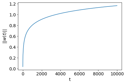
and the residual grows at most as $|\rho(t)| = O(\log \log (t))$ and so:

$\lim_{t \rightarrow \infty} \frac{w(t)}{\|w(t)\|} = \frac{\hat{w}}{\|\hat{w}\|}$

Further for almost all datasets, the residual $\rho(t)$ is bounded.

Proof Sketch: First, the exponential tail of the loss function is key for the asymptotic convergence to the max margin vector. Assume the loss function: $l(u) = e^{-u}$. For linearly separable data, we will have $\forall n: w^{T}x_n \rightarrow \infty$. If $\frac{w_t}{|w_t|}$ converges to a limit $w_{\infty}$, then one can write $w(t) = g(t) w_{\infty} + \rho(t)$ such that $g(t) \rightarrow \infty$, $\forall n: w_{\infty}^{T}x_n > 0$ and $\lim_{t \rightarrow \infty} \frac{\rho(t)}{g(t)} = 0$. The gradient becomes:

$\begin{aligned} -\nabla L(w) &= \sum_{i = 1}^n \exp(-w(t)^{T} x_n) x_n\\ &= \sum_{i = 1}^n \exp\left(-g(t)^{T} w_{\infty}^{T}x_n\right)\exp\left(-\rho(t)^{T}x_n\right)x_n \end{aligned}$

As $g(t) \rightarrow \infty$, the $\exp\left(-g(t)^{T} w_{\infty}^{T}x_n\right)$ will decay much quicker for samples with small exponents. The only samples which contribute to the gradient will be the support vectors, i.e. those with the smallest margin, $\arg\min_{n} w_{\infty}^{T}x_n$.

Looking at the negative gradient above, we see that it will become a weighted average of the support vectors. Since $|w_{\infty}| \rightarrow \infty$, the initial conditions become irrelevant and $w_{\infty}$ will become dominated by the supports vectors, as will its margin-scaled version, $\hat{w} = \frac{w_{\infty}}{\min_{n} w_{\infty}^{T}x_n}$. It follows:

$\hat{w} = \sum_{n = 1}^N \alpha_n x_n \quad \forall n \quad (\alpha_n \geq 0 \text{ and } \hat{w}^{T}x_n = 1) \quad \text{OR} \quad (\alpha_n = 0 \text{ and } \hat{w}^{T}x_n > 1)$

These are exactly the KKT conditions for hard-margin SVM.

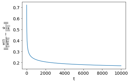
Key Theorem 2: For almost every linearly separable dataset, the normalized weight vector converges to the normalized max margin evector in $L_2$ norm:

$\left\| \frac{w(t)}{\|w(t)\|} - \frac{\hat{w}}{\|\hat{w}\|}\right\| = O\left(\frac{1}{\log t}\right)$

and in angle:

$1 - \frac{w(t)^{T}\hat{w}}{\|w(t)\| \|\hat{w}\|} = O\left(\frac{1}{\log^2 t}\right)$

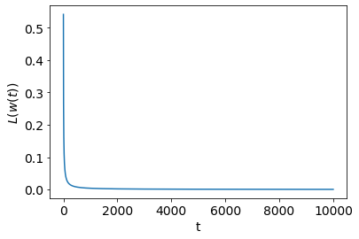
On the other hand the loss decreases as:

$L(w(t)) = O\left(\frac{1}{t}\right)$

Practical Implications:

• While the loss decreases at a fast rate towards zero, the convergence of $w(t)$ to the max-margin $\hat{w}$ is slow. You may need to wait until the loss is exponentially small in order to be close to the max-margin solution. So, continuing to optimize the training loss even after the training error is zero and training loss is very small can improve generalization. The margin can continue to grow.

• Since $w(t)$ converges to the max-margin $\hat{w}$, we expect population misclassification error to improve as $t \rightarrow \infty$. However, we have no guarantees that $\hat{w}$ will have zero population or test misclassification error. Since $|w(t)| \rightarrow \infty$, for convex loss functions, the loss for the misclassified points will increase as $t \rightarrow \infty$. More precisely, let $l(u) = \log(1 + e^{u})$ and note that $l(\alpha u) \rightarrow \alpha \max(0, -u)$ as $\alpha \rightarrow \infty$. For $w(t) \approx \hat{w} \log t$, we have:

  $\mathbb{E}[l(w(t)^{T}x)] \approx \mathbb{E}[l((\log t)\hat{w}^{T}x)] \approx (\log t) \mathbb{E}[\max(0, -\hat{w}^{T}x)] = \Omega(\log t)$

  This means that you can see the population or test loss increase even while the predictor’s generalization is improving. Practically, if you monitoring a validation set to stop training, you should look at the misclassification error, not the loss.

Connections to Other Results: AdaBoost can be formulated as a coordinate descent algorithm on the exponential loss of a linear model. With small enough step sizes, AdaBoost does converge precisely to the $L_1$ max-margin solution. For similar loss functions and the regularization path $w_{\lambda} = \arg\min L(w) + \lambda R(|w|)$ where $(R(|w|)$ is the $L_p$ norm penalty, one can show that $\lim_{\lambda \rightarrow 0} \frac{w_{\lambda}}{|w_{\lambda}|}$ is proportional to the max $L_{p}$ margin solution. These latter results are considering explicit regularization as opposed to implicit regularization induced by optimizaiton.

Extensions: The paper proves similar results for the multi-class setting with cross-entropy loss as well as neural nets where only a single weight layer is optimized and after a sufficient number of iterations the activation units stop switching.

Other Optimization Algorithms: Experimentally, these results continue to hold for SGD and momentum variants of GD. However, adaptive methods such as AdaGrad and ADAM do not converge to the max-margin $L_2$ solution.

A Quick Empirical Check: I ran a quick simulation to check if these results hold up empirically. I generated a linearly separable dataset of $N = 100$ samples and $d = 120$ features. Then, I ran unregularized logistic regression keep track of $w(t)$ along the optimization path. As expected, both the hard SVM solution and final logistic regression solution have zero training error. The first plot here shows the $L(w(t))$ which decays as $O\left(\frac{1}{t}\right)$. The second plot shows $|w(t)|$ which increases as $O\left(\log t\right)$. The last plot shows the margin gap which decays as $O\left(\frac{1}{\log t}\right)$. It is hard to eyeball the difference in $\frac{1}{t}$ and $\frac{1}{\log t}$, but I plotted those functions explicitly and they do in fact match these results.