Attention Mechanisms + Transformers

This is part 6 of my applied DL notes. They cover attention mechanisms and transformers.

Introduction

Attention mechanisms are different from FC or pooling layers since they take advantage of queries. They are a way to bias selection over values via a process called attention pooling, which measures interactions between queries and keys. The keys are paired to values.

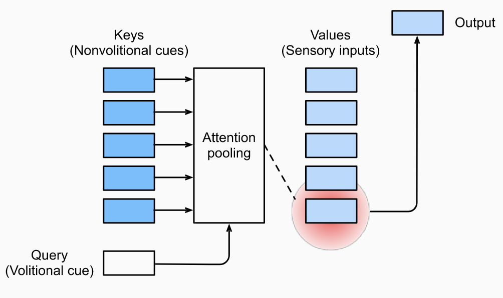
One way to think of attention pooling is by analogy to Nadraya-Watson Kernel Regression (NWKR). Consider a training dataset $(x_1, y_1), \dots (x_n, y_n)$ and a test point $(x, y)$. Then, the NWKR prediction takes the form:

$f(x) = \sum_{i = 1}^{n} \alpha(x, x_{i})y_{i}$

Here we have $x$ is the query, $x_1, \dots, x_n$ are the keys, $y_1, \dots, y_n$ are the values, and $\alpha(x, x_{1}), \dots \alpha(x, x_{n})$ are the attention weights. In NWKR, $\alpha = \frac{K(x - x_{i})}{\sum_{j}K(x - x_{j})}$ where $K$ is a kernel function. However, we can imagine that $\alpha = \alpha_{w}$. It is parameterized by a parameter $w$ which can be learned with backprop. When predicting the output of a training sample $x_{i}$, we would need to exclude it from the key-value pairs to avoid degenerate solutions for $w$.

To formally define attention mechanisms, say we have a query $q \in \mathbb{R}^{q}$ and $m$ key-value pairs $(k_1, v_1), \dots (k_m, v_m)$ where $k_i \in \mathbb{R}^k$ and $v_i \in \mathbb{R}^v$. Attention pooling $f$ is a weighted sum:

$f(q, (k_1, v_1), \dots (k_m, v_m)) = \sum_{i = 1}^{m} \alpha(q, k_i)v_i \in \mathbb{R}^v$

Here the attention weights are computed as follows:

$\alpha(q, k_i) = \text{softmax}(a(q, k_i)) = \frac{\exp(a(q, k_i))}{\sum_{k = 1}^{m} \exp(a(q, k_j))} \in \mathbb{R}$

where $a$ is a scoring function that maps two vectors to a scalar based on their similarity/importance.

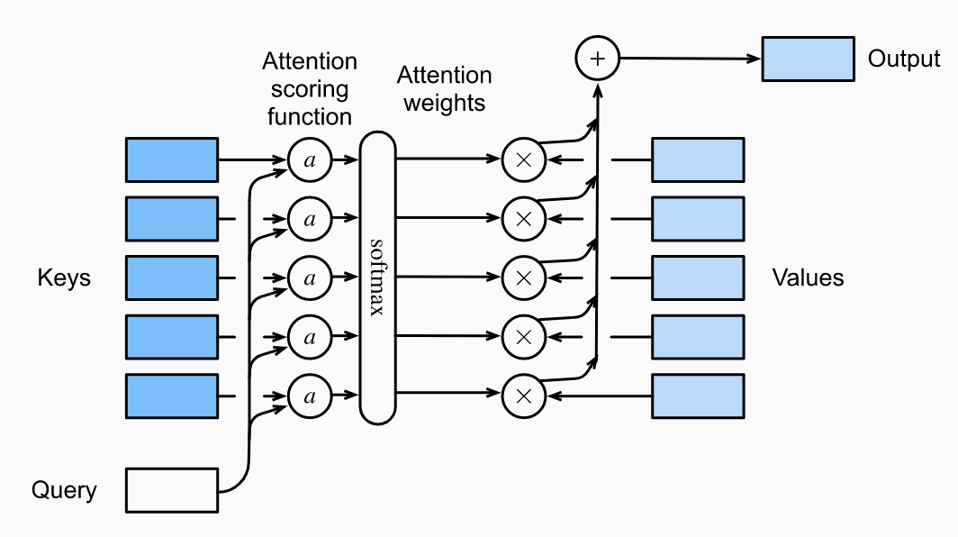
Sometimes we will want a masked softmax operation to compute the attention weights. For example, in machine translation, we often have <pad> tokens which carry no meaning and should not be fed into attention pooling. The attention weights can be visualized by producing a matrix with queries as rows, keys as columns and attention weights as values.

Scoring Functions

Additive Attention

When queries and keys are vectors of different lengths, additive attentions is given by:

$a(q, k) = w_{v}^{T} \tanh(W_{q}q + W_{k}k) \in \mathbb{R}$

where $W_{q} \in \mathbb{R}^{h \times q}$, $W_{k} \in \mathbb{R}^{h \times k}$ and $w_{v} \in \mathbb{R}^{v}$. Concatenating the query and key, we can see this equation is just a single-layer MLP, with $\tanh$ activation and no bias terms.

Scaled Dot-Product Attention

If the two vectors of the same dimension, a more computationally efficient scoring function is just the dot product. But assuming that both $k$ and $q$ are independent zero mean and unit variance vectors, $q^{T}k$ will be zero mean and variance $d$. Hence when $d$ is large and the magnitude of the dot product is large, we may end up pusing the $\text{softmax}$ into regions where it has very small gradients, making learning difficult. So, we scale:

$a(q, k) = q^{T}k / \sqrt{d}$

We will typically processes whole minibatches at time. Consider $n$ queries, $m$ key-value pairs, queries/keys of size $d$ and values of size $v$. Then, the scaled dot-product attention weights are given by:

$\text{softmax}\left(\frac{QK^{T}}{\sqrt{d}}\right)V \in \mathbb{R}^{n \times v}$

where $Q \in \mathbb{R}^{n \times d}$, $K \in \mathbb{R}^{m \times d}$ and $V \in \mathbb{R}^{m \times v}$.

Bahdanau Attention

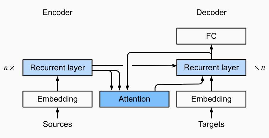
Recall our usual encoder-decoder RNN architecture uses the same context variable (which encodes the input sequence) in each decoding step. But not all input tokens may be useful for decoding a particular token. By treating the context variable as the output of attention pooling, we can get our model to align to parts of the input sequence most relevant to the current prediction.

We have the context variable at decoding time $t'$ is given by:

$c_{t'} = \sum_{t = 1}^{T} \alpha(s_{t' - 1}, h_t)h_t$

Here the decoder hidden state $s_{t' - 1}$ from time step $t' - 1$ is the query, the $T$ encoder hidden states $h_{t}$ are the key-value pairs, and we can compute $\alpha$ using the additive attention scoring function as $a$.

Implementation Notes

• For initializing the decoder, you need to do two things. First, pass in the encoder final-layer hidden states at all the time steps, so they can be used for the key-value pairs in attention. Second, as usual, pass the encoder all-layer hidden state at the final step to initialize the decoder hidden state.
• As you are running the decoder, the attention output at any step depends on the previous decoder hidden state. So, you will need to iterate over time steps one by one. Each time, you will concatenate the new attention output to the target embedding to pass through the RNN cell.

Multi-Head Attention

Given some set of queries/keys/values, it is possible we want our model to combine different types of attentions. For example, maybe we want to capture shorter and longer range dependencies within a sequence. Instead of learning a single attention pooling, the queries/keys/values can be transformed with $h$ learned linear projections. These $h$ sets of queries/keys/values are then pushed into attention pooling in parallel. Finally, these $h$ attention pooling outputs are concatenated and pushed through a FC layer to get the final output. This is called multi-head attention.

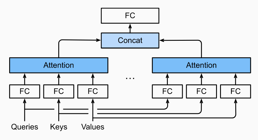
Formally, say we have a query $q \in \mathbb{R}^{d_q}$, key $k \in \mathbb{R}^{d_k}$, value $v \in \mathbb{R}^{d_v}$, each attention head $h_{i}$ for $i \in [h]$ is computed as:

$h_{i} = f(W_{i}^{(q)}q, W_{i}^{(k)}k, W_{i}^{(v)}v) \in \mathbb{R}^{p_v}$

for learnable parameters $W_{i}^{(q)} \in \mathbb{R}^{p_q \times d_q}$, $W_{i}^{(k)} \in \mathbb{R}^{p_k \times d_k}$, $W_{v}^{(k)} \in \mathbb{R}^{p_v \times d_v}$ and $f$ is attention pooling as we know from earlier. Finally, we have the output:

$W_{o} [h_1, \dots h_{h}]^{T} \in \mathbb{R}^{p_o}$

where $W_{o} \in \mathbb{R}^{p_o \times h p_v}$. In this way, each head can align with different patterns in the input sequence.

Typically, we set $p_{q} = p_{k} = p_{v} = p_{o}/h$. This helps control the computational cost and number of parameters. With the reduced dimension of each head, $p_{o}/h$, the total computational cost is similar to that of a single head with full dimensionality.

One of the key facets of multi-head attention is that it can be computed in parallel, as we will see when we look at Transformer architectures. Leveraging parallelization will require proper tensor manipulation in PyTorch.

Self-Attention

Self-attention refers to passing in the same set of tokens for queries, keys and values. To use self-attention for sequence modeling, we have to include additional information on sequence order.

Formally, self-attention is as follows. Given a set of input tokens $x_1, \dots, x_n$, self attention outputs a sequence $y_1, \dots y_n$ such that:

$y_i = f(x_{i}, (x_1, x_1), \dots, (x_n, x_n))$

where $f$ is attention pooling.

CNNs vs RNNs vs Self-Attention

To realize the benefits of self-attention, consider modeling an output sequence of $n$ tokens given an input sequence of $n$ tokens. All tokens are of dimension $d$. We compare computational complexity, sequential operations and maximum path length of CNNs, RNNs and self-attention. Recall that sequential operations will make it difficult to parallelize computation and a long maximum path length will make it difficult to learn long-range dependencies.

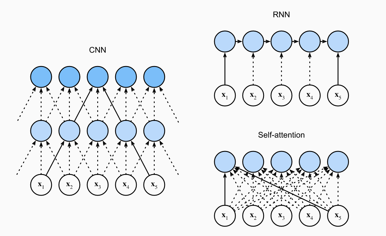
First, note that the CNNs we will have $d$ input and $d$ output channels. Note we can just think of a sequence as a $1D$ image. Then, given a kernel size $k$, the compute time is $O(knd^{2})$. The CNN operations are hierarchical, so there are $O(1)$ sequential operations. Finally, the max path length is $O(n / k)$.

For RNNs, we have to multiply a $d \times d$ weight matrix by a $d$-dimensional hidden state, which has complexity $O(d^2)$. We do this $n$ times, so the compute time is $O(n d^{2})$. There are $O(n)$ sequential operations that cannot be parallelized and the max path length is also $O(n)$.

In self-attention, all queries/keys/values are $n \times d$ matrices. We first multiply a $n \times d$ matrix by a $d \times n$ matrix. Then, we multiply the $n \times n$ output by a $n \times d$ matrix. The compute complexity is $O(n^2d)$. Each token is connected to each other token so the sequential operations are $O(1)$ and the max path length is also $O(1)$.

Hence both CNNs and self-attention can be parallelized. Self-attention has the shortest max path length, but quadratic compute complexity with regards to $n$ makes it slow for long sequences.

Positional Encoding

In self-attention, we have forgone any sequential info for the ability to parallelize. To add sequence order back to the model, we include a positional encoder along with our input embedding. The positional encoder can be learned or fixed. Here we consider a fixed one based on sin and cosines. We will generate a matrix $P \in \mathbb{R}^{n \times d}$ and instead of passing the original input embedding $X$, we will pass $X + P$. The entries as follows:

$p_{i, 2j} = \sin\left(\frac{i}{10000^{2j/d}}\right) \\ p_{i, 2j + 1} = \sin\left(\frac{i}{10000^{2j/d}}\right)$

Here each row is a position in the sequence. Each column is a trig function of some frequency. Higher order columns are lower frequencies. The intuition is as follows. Think of 0-7 in binary: 000, 001, 010, 011, 100, 101, 110, 111. Notice the last bit alternates every number; it is high frequency. The middle bit alternates every two numbers; it is lower frequency. The firs tbit alternatives every four numbers; it is the lowest frequency. So, we are basically just converting each number to binary and using a continuous representation.

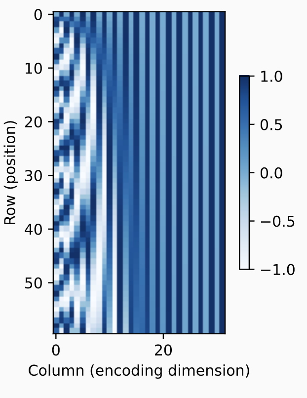
In fact one can show that in addition to telling us about absolute position, this encoding also tells us about relative position. This is beacuse the positional encoding at any position $i + \delta$ can be represented as a linear transform of the position at $i$.

Transformers

Transformers are a deep architecture which abandon any recurrent or convolutional operations in favor of self-attention. They are a go-to model for many applied DL domain areas.

An transformer architecture is below. It is an encoder-decoder architecture but either one can be used individually. The source/target embeddings go through positional encoding before being pushed through the individual stacks.

The encoder stack is $n$ layers. Each layer consists of: 1) multi-head attention and 2) a positionwise feed-forward network. In each layer, the queries/keys/values come from the previous layer output. Both sub-layers employ a residual connection. To make this feasible, for any sub-layer input $x \in \mathbb{R}^d$, we require the sub-layer output $f(x) \in \mathbb{R}^d$, so $x + f(x)$ is possible. The residual connection is followed by layer-normalization. The output of the enconder is a $d$ dimensional representation for each position in the input sequence.

The decoder stack is similar, but each layer consists of a third sublayer, encoder-decoder attention. In encoder-decoder self-attention, the queries are outputs from the previous decoder layer and the keys-value pairs are the encoder outputs. In decoder self-attention, queries/keys/values are all outputs from the previous layer, but the decoder can only align with outputs previous positions. This is called masked attention and ensures that during test time, prediction only depends on tokens which have been generated.

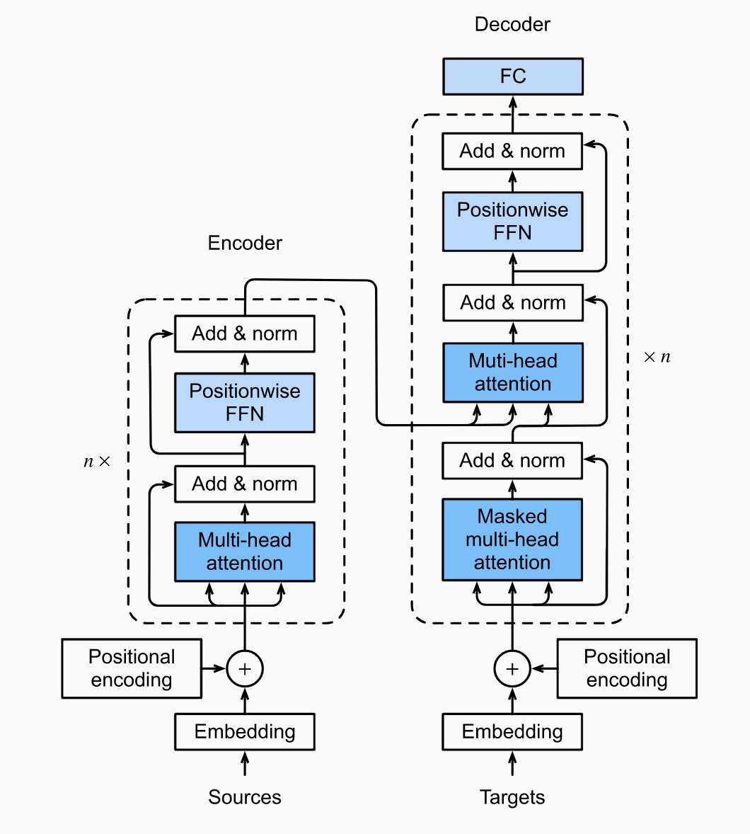
A positionwise feed-forward NN merely transforms the representation at each sequence position using the same MLP. Layer-normalization is similar to batch normalization. While batch normalization standardizes each feature across examples within a given minibatch, layer normalization standardizes each example across all of its feature dimensions. It is common in NLP.