Counterfactual Prediction with Time-Varying Treatments + G-Computation

Here I document an algorithm known as G-computation, which is a tool for doing counterfactual prediction in time series settings.

Set-up

We assume that we have $n$ iid data strings $X_{i} \sim \mathbb{P}$ where:

$X = (\bar{A}_{T}, \bar{L}_{T}, Y) = (A_1, L_1, A_2, L_2, \dots A_T, L_T, Y)$

Given the iid assumption, we suppress dependence on subject index $i$. We have a full time series, $t = 1, 2, \dots T$, for both $A_{t}$ and $L_{t}$. Here we let $\bar{A}_{t} = (A_{1}, \dots A_{t})$ and $\bar{L}_{t} = (A_{1}, \dots L_{t})$ for $t \geq 1$.

Let $A_{t}$ be a treatment variable on date t. When $A_{t} = 1$ treatment is on and when $A_{t} = 0$ treatment is off. We let $L_{t}$ denote a set of confounders on date $t$. Notice that in almost all practical settings, $L_{t}$ is actually a vector of variables, but for ease of exposition it suffices to treat it as a single variable. In the following sections, anytime we include $L_{t}$ in a regression model, just keep in mind that there are in fact multiple associated coefficients, rather than just one. Finally, $Y$ is an outcome of interest.

Because we are interested in counterfactual prediction, we denote $Y(\bar{a}_T)$ as the potential outcome when one sets $\bar{A}_{t} = \bar{a}_{t}$. If $A_{t}$ is binary, there are $2^{T}$ such quantities, one for each possible treatment regime $\bar{a}_{T}$. In general, these quantities are unobserved, while $Y$ is the observed quantity in our dataset.

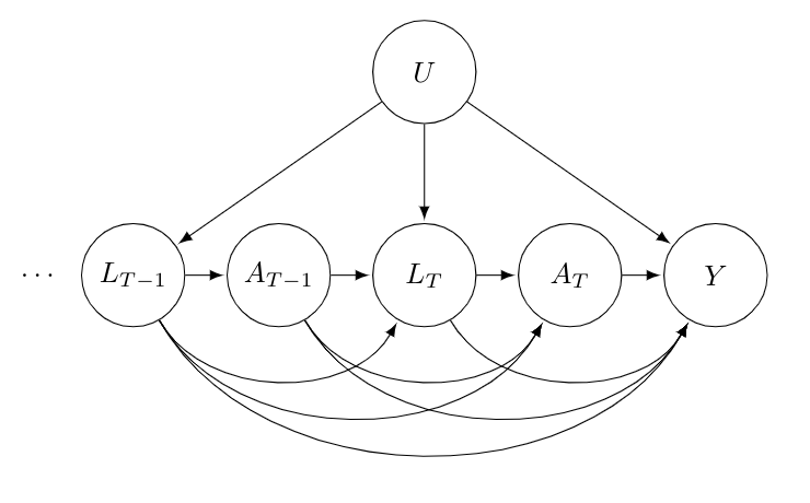
A DAG which describes the set-up above is as follows:

For simplicity, we only consider the last two periods, $T-1$ and $T$, of our data string. It is reasonable to assume that all past confounders and past treatments affect all future confounders, treatment and the final outcome. Moreover, we are dealing with observational data and have tried to measure all possible confounders. However, it is likely there are some unobserved factors, $U$, which influence the confounders, $L_{t}$, and outcome $Y_{T + 1}$. As a result, $U$ will arrows into $L_{T - 1}$, $L_{T}$ and $Y_{T + 1}$.

Why can’t we use standard regression?

An intuitive approach would be to assume a linear model as follows:

$Y = \alpha + \sum_{t = 1}^{T} \beta_t L_t + \sum_{t = 1}^{T} \omega_t A_t + \epsilon$

We could fit this with OLS and set $\hat{\mathbb{E}}[Y(\bar{a}_T)] = \hat{\mathbb{E}}[\hat{\mathbb{E}}[Y \mid \bar{L}_T, \bar{A}_T = a_T]]$. The estimated conditional expectations come from the OLS fits for particular samples. The estimated outer expectation is an average of these fits over all the samples.

The above strategy would be valid if $\bar{A}_{T} \perp Y(\bar{a}_T) \mid \bar{L}_T$. This would be similar to the usual “selection on observables” assumption made in causal inference. However, the time series dependence in our set-up makes such an assumption highly unlikely.

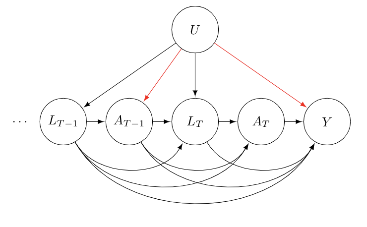
The core issue boils down to collider bias. From our DAG above, it is clear that we need to condition on $L_{T}$. It points to both $Y$ and $A_{T}$ and is thus a confounder. However, notice that both $A_{T - 1}$ and $U$ point to $L_{T}$. Thus, $L_{T}$ is a collider and including it in our regression induces a correlation between $A_{T - 1}$ and $U$. Since $U$ points to $Y$, the conditional independence statement above fails. By conditioning on $L_{T}$, our DAG now includes the path denoted by the red arrows:

In addition to collider bias, when we condition on $L_{T}$, we block a causal path of interest. Specifically, $A_{T - 1} \rightarrow L_{T} \rightarrow Y$. Thus, it seems like we need to condition on $L_{T}$ as it is a confounder, but doing so will get us biased predictions for $Y(\bar{a}_T)$.

G-Computation

A solution to the above issue is G-computation. It was originally proposed in R1986 and additional details relevant to our set-up are included in RGH1999. The key is to make the following identification assumption:

Identification Assumption: For all $t = 1, \dots T$:

$A_{t} \perp Y(\bar{a}_T) \mid (\bar{A}_{t - 1}, \bar{L}_{t})$

That is conditional on the past history of treatments and confounders, treatment at any given time is random.

Combined with the standard causal assumptions of positivity and consistency, it is possible to estimate $\mathbb{E}[Y(\bar{a}_T)]$ without bias.

Theorem: For any $\bar{a}_{T}$:

$\mathbb{E}[Y(\bar{a}_T)] = \int_{L_1} \int_{L_2} \dots \int_{L_T} \mathbb{E}[Y \mid \bar{L}_T, \bar{A}_T = a_{t}] \prod_{t = 1}^T f(L_{t} \mid \bar{L}_{t-1}, \bar{A}_{t-1} = \bar{a}_{t-1})$

Here $f$ are the conditional densities of $L_{t}$ given the past.

Proof:

$\begin{aligned} \mathbb{E}[Y(\bar{a}_T)] &= \mathbb{E}[\mathbb{E}[Y(\bar{a}_T) \mid L_{1}]]\\ &= \mathbb{E}[\mathbb{E}[Y(\bar{a}_T) \mid L_{1}, A_{1} = a_1]]\\ &= \mathbb{E}[\mathbb{E}[\mathbb{E}[Y(\bar{a}_T) \mid L_{1}, L_{2}, A_{1} = a_1] \mid L_{1}, A_{1} = a_1]]\\ &= \mathbb{E}[\mathbb{E}[\mathbb{E}[Y(\bar{a}_T) \mid \bar{L}_{2}, \bar{A}_2 = \bar{a}_2] \mid L_{1}, A_{1} = a_1]]\\ &= \mathbb{E}[\mathbb{E}[\mathbb{E}[\mathbb{E}[Y(\bar{a}_T) \mid \bar{L}_3, \bar{A}_2 = \bar{a}_2] \mid \bar{L}_{2}, \bar{A}_2 = \bar{a}_2] \mid L_{1}, A_{1} = a_1]]\\ &= \mathbb{E}[\mathbb{E}[\mathbb{E}[\mathbb{E}[Y(\bar{a}_T) \mid \bar{L}_3, \bar{A}_3 = \bar{a}_3] \mid \bar{L}_2, \bar{A}_2 = a_2] \mid L_{1}, A_{1} = a_1]]\\ &= \dots \\ &= \mathbb{E}[ \dots \mathbb{E}[\mathbb{E}[Y(\bar{a}_T) \mid \bar{L}_{T}, \bar{A}_{T} = \bar{a}_{T}] \mid \bar{L}_{T - 1}, \bar{A}_{T - 1} = \bar{a}_{T - 1}] \dots \mid L_{1}, A_{1} = a_1]]\\ &= \mathbb{E}[ \dots \mathbb{E}[\mathbb{E}[Y \mid \bar{L}_{T}, \bar{A}_{T} = \bar{a}_{T}] \mid \bar{L}_{T - 1}, \bar{A}_{T - 1} = \bar{a}_{T - 1}] \dots \mid L_{1}, A_{1} = a_1]]\\ &= \int_{L_1} \int_{L_2} \dots \int_{L_T} \mathbb{E}[Y \mid \bar{L}_T, \bar{A}_T = a_{t}] \prod_{t = 1}^T f(L_{t} \mid \bar{L}_{t-1}, \bar{A}_{t-1} = \bar{a}_{t-1}) \end{aligned}$

The steps here rely on repeated application of the law of total expectation and then the key identification assumption above. The second to last equality relies on consistency. The last equality relies on positivity which ensures that the integrand can be evaluated for all possible values $A_{t}$ and $L_{t}$.

A natural estimator $\mathbb{\hat{E}}[Y(\bar{a}_T)]$ is to simply plugin a fitted outcome model $\mathbb{\hat{E}}[Y \mid \bar{L}_T, \bar{A}_T = a_{t}]$ and conditional density estimators $\hat{f}(L_{t} \mid \bar{L}_{t - 1}, \bar{A}_{t - 1} = \bar{a}_{t - 1})$ learned from one’s data. A standard parametric approach would be to use GLMs and make a Markov assumption to limit the number of lags. Non-parametric methods ranging from kernel smoothers to modern ML methods can also be used here. Correctly specified parametric models will typically imply convergence to the truth at a $\sqrt{n}$-rate and normal limiting distributions. Nice convergence properties for general non-parametric methods are not as easily guaranteed, but do hold under specific smoothness assumptions. In all cases, standard errors can be evaluated via the bootstrap.

In general, when using non-linear models, the integral is intractable to compute analytically. Instead, one relies on a Monte Carlo simulation. Specifically, for $i \in [N]$, where $N$ is the number of simulation samples, one does the following:

1. For $t \in [T]$:

   a. Set $A_{t} = a_t$

   b. Draw $L_{t} \sim \hat{f}(L_{t} \mid \bar{L}_{t - 1}, \bar{A}_{t - 1} = \bar{a}_{t - 1})$

2. Set $\hat{Y}_{i}(\bar{a}_T) = \hat{\mathbb{E}}[Y \mid \bar{L}_T, \bar{A}_T = \bar{a}_{t}]$

Then, $\hat{\mathbb{E}}[Y(\bar{a}_T)] = \frac{1}{N} \sum_{i = 1}^{N} \hat{Y}_i(\bar{a}_T)$. To get standard errors, we generate $B$ bootstrap samples and the whole algorithm is re-run starting with fitting the the outcome model and conditional density estimators.

Marginal Structural Models

An alternative to G-computation is to use marginal structural models which posit a specific parametric form for $\mathbb{E}[Y(\bar{a}_T)] = g(\bar{a}_T, \beta)$ and use IPW estimators of $\beta$. Non-parametric G-computation always implies a particular form of a MSM. Hence if the models are correctly specified, both techniques should provide the same answers. So, as a robustness check one should always try to fit both to make sure the results are similar. If not, one of the models is incorrectly specified. In the parametric case, this equivalence does not hold. There is an issue with parametric G-computation known as the “null paradox”: there may be no setting for one’s parametric models which accommodate the case where the outcome is conditionally dependent on past treatment but has no effect. Hence if you think you are in a regime where the treatment has no effect and non-parametric models seem infeasible (i.e. you have a small or very noisy sample), you should use MSMs. Finally, there are doubly-robust MSM approaches which may be useful in case you are worried about model specification or think you can model propensity scores well.