RNNs

This is part 5 of my applied DL notes. They will cover high-level intuition about RNNs and some practical advice on using them for language modeling/machine translation.

Language Modeling

One of the primary applications of RNNs is for language modeling. The goal is to learn the joint probability of a text sequence $P(x_{1}, x_{2}, \dots x_{T})$. This enables us to do text generation with $x_{t} \sim P(x_{t} \mid x_{t - 1}, \dots x_{1})$. Here are some practical insights which motivate and set-up using RNNs for this task:

• Processing:
  • Tokenize corpus into words or chars
  • Build a vocabulary which is a mapping between words and numerical indices
  • Keep a token to represent “unknown” in your vocabulary
  • Keep reserved tokens for end of sequence, start of sequence and padding
  • Maybe get rid of very rare tokens?
• Learning a language model $p(x_1, x_2, \dots, x_{T})$ for the sequence $x_1, \dots x_{T}$ by factorizing the joint distribution as $p(x_1)p(x_2 \mid x_1)p(x_3 \mid x_2, x_1) \dots$ and using counting estimators is not optimal because: 1) we have to store the counts, 2) ignores meaning of words, 3) long combinations of words become rare or non-existent, so modeling the tail of the frequency distribution becomes difficult.
• We can make weaker Markov assumptions to model longer dependences. We can go from unigram to n-gram models.
• Unigram, bigram, trigams all obey frequencies as $n_{i} \propto 1/i^{\alpha}$, i.e. linear on the log-log scale. This very rapid/consistent decay implies there is structure we should be able to learn with NNs.
• We will need to split up very large sequences into smaller sub-sequences for modeling in a NN. Assume that each minibatch has to contain samples with $n$ time steps. We can:
  • Use random sampling. We truncate the long sequence before a random offset and then randomly shuffle the possible starting points for the smaller $n$-step subsequences. Two examples in the minibatch may not be adjacent in the original text.
  • Sequential partitioning. Again, we use a random offset, but then do not shuffle the starting points.

Perplexity

Say a language model is completing a sequence “It is raining … “. A model which completes it with “outside” is better than “asdasdsad”. We can compute the likelihood of “It is raining outside” and see it is higher than “It is raining asdasdsad.” It is hard to evaluate likelihoods, especially since longer sequences will be less likely. We need an average. Hence it is reasonable to use perplexity:

$\exp\left(-\frac{1}{n} \sum_{t =1}^{n} \log P(x_{t} \mid x_{t - 1}, \dots x_{1})\right)$

Here $P$ is given by a language model and $x_{t}$ is the actual token at time $t$. So, this is the exponential of the cross entropy entropy loss average over the $n$ tokens. If our model is perfect, perplexity is 1. In our model always completely wrong, perplexity is $\infty$. A model which predicts uniform over the tokens in a vocab will have a perplexity of the number of unique tokens. Intuitively, perplexity tells us a better language model is able to spend fewer bits to compress the sequence.

Machine Translation

Machine translation is a related, but different problem. The goal is to map an input sequence in one language to an output sequence in another language. The text processing is much the same, but there are a few differences:

• We have two vocabularies.
• We can have variable-length inputs/outputs. To ensure that all sequences in a minibatch are the same length, we can fix a given length of $n$ time steps. Sequences that are too small can be padded with a <pad> token. Sequences that are too long can be truncated.
• It will be useful to add a <eos> token to indicate the end of a sequence to indicate the end of an input sequence or keep track of the true lengths. Similarly, we can add <bos> tokens.

BLEU

For machine translation, the performance metric is usually BLEU. For any $n$-gram in the predicted sequence, BLEU evaluates whether this $n$-gram appears in the label truth. We denote $p_{n}$ as the ratio of the number of matched $n$-grams to the number of $n$-grams in the predicted sequence. For example, given a predicted sequence ABBCD and a label sequence ABCDEF, we have $p_{1} = 4/5, p_{2} = 3/4, p_{3} = 1/3$ and $p_{4} = 0$. Then, BLEU is:

$\exp\left(\min\left(0, 1 - \frac{\text{len}_{\text{label}}}{\text{len}_{\text{pred}}}\right)\right)\prod_{n = 1}^{k} p_{n}^{1/2^{n}}$

where $k$ is the longest $n$-grams for matching. If the predicted sequence exactly equals the label sequence, we have BLEU is 1. Also, since $p_{n}^{1/2^{n}}$ grows with $n$ for a fixed $p_{n}$, BLEU assigns greater value to longer $n$-gram precision. Finally, since predicting shorter sequences will get you higher $p_{n}$, the $\exp(\cdot)$ term penalizes shorter predicted sequences.

RNNs

Assume a $n$-gram model where the conditional probability of a word at time step $t$ only depends on the last $n - 1$ words. For a vocab $\mathcal{V}$, a counting model model would need to store $\lvert \mathcal{V} \rvert^{n}$ numbers. Instead, we can use a latent variable model:

$P(x_{t} \mid x_{t - 1}, \dots x_{1}) \approx P(x_{t} \mid h_{t - 1})$

where $h_{t - 1}$ is a hidden state that summarizes information through time $t - 1$. We can let $h_{t} = f(x_{t}, h_{t - 1})$. Note we want $h_{t}$ to be a small, but useful representation of the past time steps. It should not just store the full sequence; that would be infeasible memory/compute-wise. RNNs are NNs with hidden states. Let $X_{t} \in \mathbb{R}^{n \times d}$ be a minibatch of inputs at time $t$ and $H_{t} \in \mathbb{R}^{n \times h}$ be the hidden state at time $t$. We have $H_{t - 1} \in \mathbb{R}^{n \times h}$ stored from the last step. We model:

$H_{t} = \phi(X_{t}W_{xh} + H_{t - 1}W_{hh} + b_{h})$

So, the hidden state today depends on its dependence on to the hidden state yesterday, parameterized by $W_{hh}$, and its dependence on the input today, parameterized by $W_{xh}$. Finally, we generate the output $O_{t} \in \mathbb{R}^{q}$ as:

$O_{t} = H_{t}W_{hq} + b_{q}$

Note that the weights $W_{xh}, W_{hh}, W_{hq}, b_{h}$ and $b_{q}$ are constant across time steps. So, parameterization does not increase with $t$. Note we can simplify computation of $H_{t}$ here by concatenating the matrices into $[X_{t}, H_{t - 1}] \in \mathbb{R}^{n \times (d + h)}$ and feeding them into a FC “hidden state” layer paramterized by $[W_{xh}, W_{hh}] \in \mathbb{R}^{(d + h) \times h}$. Then, we take $H_{t}$ and feed it into a FC “output” layer parameterized by $W_{hq}$ to get $O_{t}$.

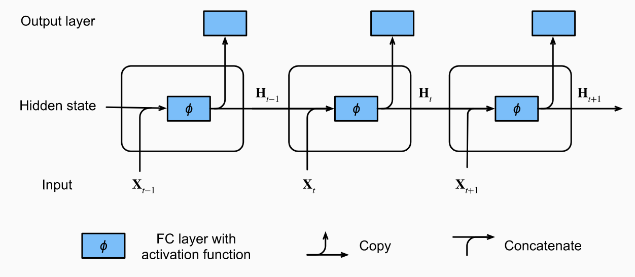
RNNs for Character-Level Language Models

As a concrete example, consider the character RNN below where we want to predict the next token using current and past tokens. Consider a minibatch of size 1 with the sequence given by “machine.” In step 3, $O_{3}$ depends on “mac” and the cross-entropy loss will depend on the $\text{softmax}(O_{3})$ and the true char “h.” In practice, each token is a vector and batch size is greater than 1. So, the input is $X_{t} \in \mathbb{R}^{n \times d}$.

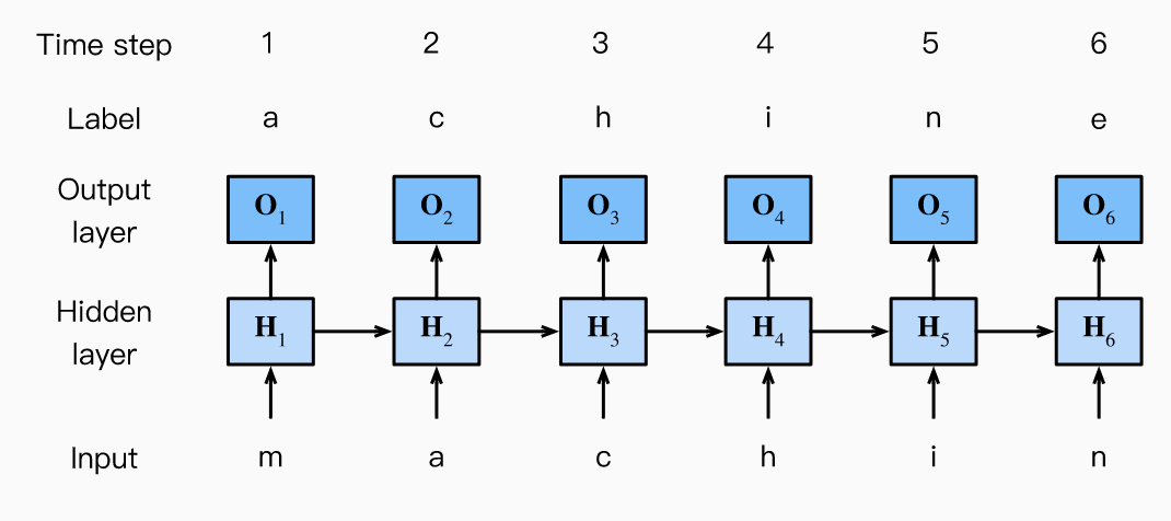
Some implementation advice:

• Recall we build a numerical index map for each token. Feeding indices to the NN might make it hard to learn. Instead, we choose an embedding representing each token as a feature vector. The easiest one is one-hot encoding. Alternatively, this can be a learned matrix where the rows are of length vocab size and the columns are of length embedding dimension. In PyTorch, a nn.Embedding layer is just a map which fetches the $i$th row from the matrix given input token $i$.
• It is easiest to reshape your tensors to (num_steps, batch_size, dim), so you can conveniently loop through the outermost dimension to update hidden states and generate outputs.
• During prediction, you may be given a user-supplied prefix. You should use these prefixes in a warm-up period to update your hidden state, so it is better than initialization.
• For training: If you use sequential partitioning, initialize the hidden state $H_{0}$ only the beginning of each epoch because subsequences passed in minibatches are adjacent. However, then the hidden state depends on all the past minibatches in an epoch, which complicates the gradient computation. To simplify, we detach the gradient before processing each minibatch, so it only depends on the steps in the current batch. For random sampling, we re-initialize the hidden state for each iteration since each example is in random position.
• In PyTorch, the nn.RNN Layer returns an output and an updated hidden state, where the output is not actually the final output layer computation. It is just $H_{t}$ for $t \in [1, T]$. You need an nn.Linear layer on top of it to get the actual outputs $O_{t}$.

Backprop Through Time

Backprop through time is just backprop for RNNs. There is nothing conceptually different, but it is worth studying the computational graph to point out potential issues we run into with long sequences.

Think about a sequence with $T = 1000$. The first token can potentially influence the last token. Computing and storing the gradients of can then take too long and requires to much memory. Moreover, it will typically be numerically unstable. To be more mathematically precise, consider an RNN with the identity activation and no bias parameters. For time step $t$, let a single example input be $x_{t} \in \mathbb{R}^d$, label $y_{t}$, hidden state $h_{t} \in \mathbb{R}^{h}$ and output $o_{t} \in \mathbb{R}^{q}$. Then we have:

$h_{t} = W_{hx}x_{t} + W_{hh}h_{t - 1}$

$o_{t} = W_{qh}h_{t}$

If the loss at time $t$ is $l(o_{t}, y_{t}$, the objective function is:

$L = \frac{1}{T}\sum_{t} l(y_{t}, o_{t})$

The computational graph below shows the dependencies. Following the arrows backwards from $L$ to parameters $W_{hx}, W_{hh}$ and $W_{qh}$, we can get the gradients of interest.

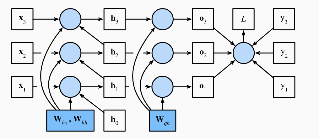
First, we have:

$\frac{\partial L}{\partial o_{t}} = \frac{1}{T} \frac{\partial l(o_{t}, y_{t})}{\partial o_{t}} \in \mathbb{R}^{q}$

Since $L$ depends on $W_{qh}$ through $o_{1}, o_{2}, \dots, o_{T}$, the chain rule for total derivatives gives us:

$\frac{\partial L}{\partial W_{qh}} = \sum_{t} \text{prod}\left(\frac{\partial L}{\partial o_{t}}, \frac{\partial o_{t}}{\partial W_{qh}} \right) = \sum_{t} \frac{\partial L}{\partial o_{t}} h_{t}^{T} \in \mathbb{R}^{q \times h}$

For the final time step $T$, we have $L$ only depends on $h_{T}$ through $o_{T}$:

$\frac{\partial L}{\partial h_{T}} = \text{prod}\left(\frac{\partial L}{\partial o_{t}}, \frac{\partial o_{t}}{\partial h_{T}} \right) = W_{qh}^{T} \frac{\partial L}{\partial o_{t}} \in \mathbb{R}^{h}$

For $t < T$, it is more complicated as $L$ depends on $h_{t}$ through $o_{t}$ and $h_{t + 1}$:

$\frac{\partial L}{\partial h_{t}} = \text{prod}\left(\frac{\partial L}{\partial h_{t + 1}}, \frac{\partial h_{t + 1}}{\partial h_{t}}\right) + \text{prod}\left(\frac{\partial L}{\partial o_{t}}, \frac{\partial o_{t}}{\partial h_{t}}\right) = W_{hh}^{T} \frac{\partial L}{\partial h_{t + 1}} + W_{qh}^{T} \frac{\partial L}{\partial o_{t}}$

Unrolling the recursion, we get:

$\frac{\partial L}{\partial h_{t}} = \sum_{i = t}^{T} (W_{hh}^{T})^{T - i} W_{qh}^{T} \frac{\partial L}{\partial o_{T + t - i}} \in \mathbb{R}^{h}$

Here we see for long sequence models we are going to have very large powers of $W_{hh}^{T}$. Eigenvalues smaller than 1 will vanish, while eigenvalues greater than 1 will diverge. We have numerical instability which will cause either vanishing/exploding gradients. Finally, notice that $L$ depends on $W_{hx}$ and $W_{hh}$ through hidden states $h_{1}, \dots h_{T}$, so we get:

$\frac{\partial L}{\partial W_{hx}} = \sum_{t} \text{prod}\left(\frac{\partial L}{\partial h_{t}}, \frac{\partial h_{t}}{\partial W_{hx}} \right) = \sum_{t = 1}^{T} \frac{\partial L}{\partial h_{t}} x_{t}^{T} \in \mathbb{R}^{h \times d}$

$\frac{\partial L}{\partial W_{hh}} = \sum_{t} \text{prod}\left(\frac{\partial L}{\partial h_{t}}, \frac{\partial h_{t}}{\partial W_{hh}} \right) = \sum_{t = 1}^{T} \frac{\partial L}{\partial h_{t}} h_{t - 1}^{T} \in \mathbb{R}^{h \times h}$

Again, any numerical instability from $\frac{\partial L}{\partial h_{t}}$ quantity will show up in both $\frac{\partial L}{\partial W_{hh}}$ and $\frac{\partial L}{\partial W_{hx}}$.

Training an RNN is the same as any other NN. We alternate between forward passes and backprop through time. Any intermediate values are cached, i.e. $\frac{\partial L}{\partial h_{t}}$ is stored in memory to compute $\frac{\partial L}{\partial W_{hh}}$ and $\frac{\partial L}{\partial W_{hx}}$.

Strategies to Handle Numerical Instability

First, we could do the full backprop computation. But then we are giving up on finding robust models which will generalize well. As a result of the instability, small perturbations in initial conditions can lead to vastly different updates and hence final models.

Second, we can truncate the summation in $\frac{\partial L}{\partial h_{t}}$ after some $\tau$ number of steps. For example, one could detach the gradient after a given number of time steps or between mini-batches. The model focuses on short-term influences rather than long-term influences. People have found this bias is desirable as it leads to simpler, more stable models.

A more complicated truncation approach is randomized. Specifically, define a sequence $\epsilon_{t}$ with parameter $0 \leq \pi_{t} \leq 1$ where $P(\epsilon_{t} = 0) = 1 - \pi_{t}$ and $P(\epsilon_{t} = \pi_{t}^{-1}) = \pi_{t}$, so $\mathbb{E}[\epsilon_{t}] = 1$. We then define:

$z_{t} = \epsilon_{t} W_{hh}^{T} \frac{\partial L}{\partial h_{t + 1}} + W_{qh}^{T} \frac{\partial L}{\partial o_{t}}$

Notice that $\mathbb{E}[z_{t}] = \frac{\partial L}{\partial h_{T}}$, but whenever $\epsilon_{t} = 0$, we do not unroll the recursion. So, only rarely do we get very long chain rule sequences. By re-weighting long sequences up in a clever manner, one can get such a scheme to provide unbiased gradient estimates.

From bottom up, the picture shows these three strategies for analyzing the few words of a text. In practice, the regular truncation works best. It sufficiently captures the relevant dependencies, it is lower variance than the randomized strategy and has a desirable regularization effect.

Gradient Clipping

In RNNs, a well-known issue is unstable optimization. For a sequence length of $T$, the gradient will involve a chain of matrix-products of length $O(T)$ during backprop. Since this product involves the same matrices over and over again, we can have the vanishing/exploding gradients problem.

One issue you can face is that once in a while your gradients can get too large and your algorithm diverges. A reasonable approach to use gradient clipping:

$g \leftarrow \min\left(1, \frac{\theta}{\|g \|}\right)g$

So, now $\|g\| \leq \theta$ and the gradient points in the original direction. It also has the nice side-effect of robustifying optimization to a given minibatch or particular sample. Sometimes people do compute the gradient norm over all the parameters in the sample.

Gated Recurrent Units (GRU)

We know that long products of matrices can lead to vanishing/exploding gradients. To get better control of our gradients, we may want to add the ability to: store early vital info which otherwise would need a large gradient to exert influence, slip irrelevant tokens and forgetting our internal state representation when there is a logical break in the sequence.

To address these concerns, GRUs support gating of the hidden state. Specifically, it introduces learned mechanisms for when a hidden state should be updated and when it should be reset.

Reset and Update Gates

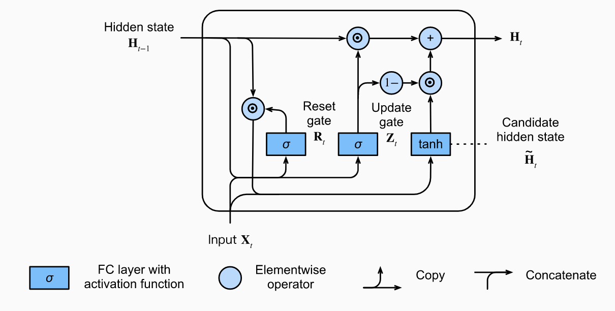
Consider a mini-batch of $n$ samples. Reset gates, $R_{t} \in \mathbb{R}^{n \times h}$, will help capture short-term dependencies in sequences. Update gates, $Z_{t} \in \mathbb{R}^{n \times h}$, will help capture long-term dependencies in sequences. They are computed as follows:

$R_{t} = \sigma(X_{t} W_{xr} + H_{t - 1} W_{hr} + b_{r})$

$Z_{t} = \sigma(X_{t} W_{xz} + H_{t - 1} W_{hz} + b_{z})$

The sigmoid functions transform the input values to vectors with entries in $(0, 1)$. This will let perform convex combinations, i.e. treat the values as weights.

Candidate Hidden States

The reset gate $R_{t}$ controls how much of the previous state we might still want to remember. It gets combined with the regular hidden state updating mechanism to get the following candidate hidden state $\tilde{H}_{t} \in \mathbb{R}^{n \times t}$:

$\tilde{H}_{t} = \tanh(X_{t}W_{xh} + (R_{t} \odot H_{t - 1}) W_{hh} + b_{h})$

The $\tanh$ ensures the values remain in the interval $(-1, 1)$. Notice that if $R_{t} \approx 0$, then $\tilde{H}_{t}$ is just an MLP result with the input $X_{t}$. The pre-existing state is reset! If $R_{t} \approx 1$, we recover the original RNN set-up. This is a candidate hidden state because we still have no accounted for $Z_{t}$.

Hidden State

The updated gate $Z_{t}$ will control how much of the new state is just a copy of the old state and to what degree the new candidate state is used. We get:

$H_{t} = Z_{t} \odot H_{t - 1} + (1 - Z_{t}) \odot \tilde{H}_{t}$

When $Z_{t} \approx 1$, the new candidate state is irrelevant and we just keep the old state $H_{t - 1}$. So, information in $X_{t}$ is ignored, effectively skipping time $t$ in the dependency chain. Whn $Z_{t} \approx 0$, the new candidate state is all that matters. This flexibility can help us solve vanishing gradient problems and capture long-run dependencies. If $Z_{t} \approx 1$ for a while, the hidden state close to the beginning can easily be retained and passed down the subsequence.

Long Short-Term Memory (LSTM)

LSTMs much like GRUs care about long-term information preservation and short-term input skipping.

Gated Memory Cell

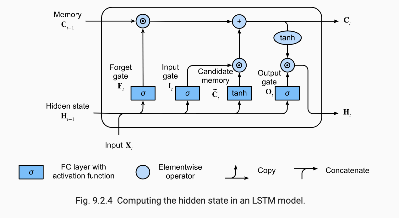
A memory cell records additional information about when to remember and when to ignore inputs in the hidden state. However, it is not passed to the output layer. It exists exclusively for state control. In it, we have the input gate $I_{t} \in \mathbb{R}^{n \times h}$ (decides when to read data into the cell), forget gate $F_{t} \in \mathbb{R}^{n \times h}$ (decides to reset the cell) and output gate $O_{t} \in \mathbb{R}^{n \times h}$ (reads entries out from th cell).

$I_{t} = \sigma(X_{t} W_{xi} + H_{t - 1} W_{hi} + b_{i})$

$F_{t} = \sigma(X_{t} W_{xf} + H_{t - 1} W_{hf} + b_{f})$

$O_{t} = \sigma(X_{t} W_{xo} + H_{t - 1} W_{ho} + b_{o})$

Notice all these values are in $(0, 1)$ due to the sigmoids. The candidate memory cell is given by:

$\tilde{C}_{t} = \tanh(X_{t}W_{xc} + H_{t - 1} W_{hc} + b_{c})$

Now, the input gate will govern how much we take new data into account via $\tilde{C}_{t}$ and the forget gate address how much of the old memory cell content $C_{t - 1}$ we retain. We get:

$C_{t} = F_{t} \odot C_{t - 1} + I_{t} \odot \tilde{C}_{t}$

Hence if $F_{t} \approx 1$ and $I_{t} \approx 0$, the past memory cells $C_{t - 1}$ will be saved over time and passed to the current time step. This captures long-run dependencies and solves the vanishing gradient problem.

Hidden State

THe output gate finally comes into play for the hidden state. We have:

$H_{t} = O_{t} \odot \tanh(C_{t})$

Notice that the values of $H_{t}$ are always in $(-1, 1)$. When $O_{t} \approx 1$, we pass all the info from the memory cell into the predictor. Else if $O_{t} \approx 0$, we retain all the info within the memory cell.

Deep RNNs

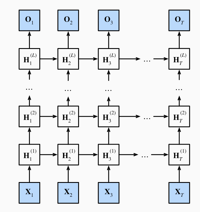
All the RNNs above have a single unidirectional hidden layer. GRUs and LSTMs specify how the inputs and latent variables interact within the hidden layer in different ways. Such specifications can be fairly arbitrary. But to create even more flexibility, we can stack several hidden layers on top of each other. Intuitively, we may think particular types of information is relevant at different levels of the stack. For example, maybe higher levels record macro-level trends, while the lower-levels keep track of shorter-term dynamics.

In a deep RNN with $L$ hidden layers, each hidden state is passed both to the next time step of the current layer and the current time step of the next layer. For simplicity, consider RNNs. For each hidden layer $l \in [L]$, we have:

$H_{t}^{(l)} = \phi_{l}(H_{t}^{(l - 1)} W_{xh}^{(l)} + H_{t - 1}^{(l)} W_{hh}^{(l)} + b_{h}^{(l)})$

Here we have $H_{t}^{(0)} = X_{t}$, $W_{xh}^{(l)} \in \mathbb{R}^{h \times h}$ and $W_{jh}^{(l)} \in \mathbb{R}^{h \times h}$. The calculation at the output layer just depends on the last hidden layer:

$O_{t} = H_{t}^{(L)} W_{hq} + b_{q}$

By simply replacing the hidden state computation with GRUs or LSTMs, we can get a deep gated RNN. Overall, ensuring proper convergence of deep RNNs requires careful settings for the learning rate, proper initialization and gradient clipping.

Bidirectional RNNs

Most sequence learning problems, we want to model the next output given what we have seen so far. But there are problems where we may see the future and want to infer the past. For example, consider fill-in-the-blank tasks where longer-range context may be useful. In HMMs, one can combine forward and backward recursions to infer $P(y_{j} \mid y_{-j})$ where $y_{i}$ form a sequence of outputs generated from hidden states $h_{i}$. We can similarly learn from the future with bidirectional RNNs.

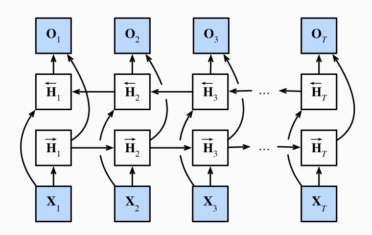
Instead of only running an RNN in forward mode from $X_{1} \rightarrow X_{T}$, we also run an RNN in reverse from $X_{T} \rightarrow X_{1}$. Another hidden layer is added to process information in the backward direction more flexibly. Formally, the forward and backward hidden states are given by $\overset{\rightarrow}{H_{t}} \in \mathbb{R}^{n \times h}$ and $\overset{\leftarrow}{H_{t}} \in \mathbb{R}^{n \times h}$. We have:

$\overset{\rightarrow}{H_{t}} = \phi(X_{t} W_{xh}^{(f)} + \overset{\rightarrow}{H_{t - 1}}W_{hh}^{(f)} + b_{h}^{(f)})$

$\overset{\leftarrow}{H_{t}} = \phi(X_{t} W_{xh}^{(b)} + \overset{\leftarrow}{H_{t - 1}}W_{hh}^{(b)} + b_{h}^{(b)})$

Next, one concatenates $\overset{\rightarrow}{H_{t}}$ and $\overset{\leftarrow}{H_{t}}$ to get the hidden state $H_{t} \in \mathbb{R}^{n \times 2h}$ which is fed to the output layer. We have:

$O_{t} = H_{t}W_{hq} + b_{q}$

where $W_{hq} \in \mathbb{R}^{2h \times q}$. In deep bidirectonal RNNs, you can pass the hidden states as inputs the next forward/backward layers. Also, the two directions can have different numbers of hidden units.

If you train a bidirectional RNN and then test it on a next token prediction problem, you will see poor performance. The model only has access to past data, but its parameters were optimized for having both future/past data. Training these models is also very slow because the forward pass requires both forward and backward recursions and backprop depends on these values creating gradients with long dependency chains.

RNN Encoder-Decoder Architecture

For modeling input/output sequences, an encoder-decoder architecture makes sense. The encoder takes the variable-length input and maps it to a fixed length state. The decoder takes this fixed length state and transforms it to a variable-length output.

For machine translation, the encoder and decoders are typically RNNs. Info on the input sequence is encoded in the hidden state of the RNN encoder. A RNN decoder generates the output token by token based on the tokens it has seen/generated plus the hidden state from the RNN encoder. Below there are two special design decisions regarding the start of the RNN decoders. First, there is a <bos> token used as an input. Second, usually the final RNN encoder hidden state is used to initiate the hidden state of the RNN decoder. Here it is taken as an input in all time steps. Notice the RNN decoder can stop making predictions once it generates <eos>. Here the labels are just the original output sequence shifted by one token.

Encoder

More precisely, the encoder transforms the input sequence into a fixed-shape context variable $c$:

$c = q(h_1, h_2, \dots, h_{T})$

using an RNN. Taking $q(h_1, h_2, \dots, h_{T}) = h_{T}$ would mean the context variable is just the final hidden state. If one used an LSTM, $c$ would include both the hidden state as well as memory cell. In one used a GRU, $c$ would just be the hidden state.

Decoder

We can think of the decoder as modeling $P(y_{t'} \mid y_{1}, \dots y_{T'}, c)$ where $y_{1}, \dots y_{T'}$ is the output sequence. At each time step $t'$, the RNN takes $c$, the previous hidden state $s_{t' - 1}$ and the previous output $y_{t' - 1}$, transforming them into the new hidden state $s_{t'}$. We have:

$s_{t'} = g(c, s_{t' - 1}, y_{t' - 1})$

After obtaining $s_{t'}$, we can use an output layer plus softmax operation to compute $P(y_{t'} \mid y_{1}, \dots y_{T'}, c)$.

Implementation Details

• To initialize the hidden state of the RNN decoder with the final hidden state of the RNN encoder, we have to ensure both of them have the same number of layers and hidden units.
• To have the context included in the all RNN decoder time steps, we have to concatenate it to all the decoder inputs.
• In addition to the context, there is some flexibility on what to pass as decoder input during training. We could pass a concatenation <bos> and the original output sequence excluding the last token. This is called teacher forcing. Alternatively, we could also pass the predicted token from the last step as input to the current step. During test, we do not have access to the original output sequence, so we have to just past the last predicted token. The test time process is shown below.

• You do not want the padded tokens to affect your loss function, so you use a mask option which zeros out irrelevant entries.

Output Sequence Search Strategies

In machine translation, we are interested in a search problem for the output sequence. Say the maximum output sequence length is $T'$. Given an output vocabulary of $\lvert \mathcal{Y} \rvert$, the goal is search from the ideal sequence in a universe of $\lvert \mathcal{Y} \rvert^{T'}$ sequences. The actual outputs will remove the portion including and after the <eos> token.

Greedy Search

In greedy search, we generate the output sequence by setting the output at each time step $t'$ with the following rule:

$y_{t'} = \arg \max_{y \in \mathcal{Y}} P(y \mid y_{1}, \dots, y_{t' - 1}, c)$

Once <eos> token is generated or the length of the output sequence reaches $T'$, the sequence is done. The optimal sequence is the sequence with the maximum value for $\prod_{t' = 1}^{T'} P(y_{t'} \mid y_{1}, \dots, y_{t' - 1}, c)$. However, greedy search is not guaranteed to return this optimal sequence.

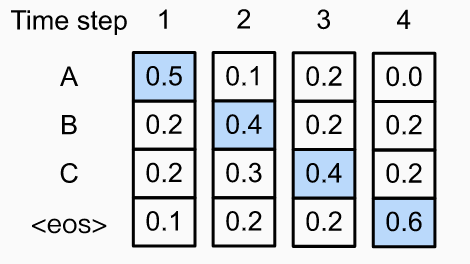
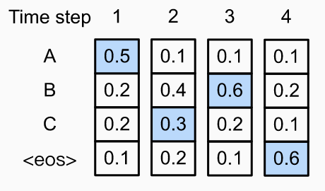
Consider the example below. Both images show the time steps on the horizontal axis and the conditional probs on the y-axis. The blue boxes are possible outputs. In the first case, the output is ABC<eos> with prob $0.5 \cdot 0.4 \cdot 0.5 \cdot 0.6 = 0.048$. This is the choice selected by greedy search. In the second case, the output is ACB<eos>. Because the second output char is different, the conditional probs of the later time steps changes. The prob here is $0.5 \cdot 0.3 \cdot 0.6 \cdot 0.6 = 0.054$, so it is better than the first choice.

Exhaustive Search

Exhaustive search will be computationally infeasible since it requires evaluating the probs of all sequences. Notice that greedy search only has a complexity of $O(\lvert \mathcal{Y} \rvert T')$ which is much better than $O(\lvert \mathcal{Y} \rvert^{T'})$.

Beam Search

Beam search can optimize the tradeoff between accuracy and computational cost. There is a hyperparameter, $k$, called beam size. At time step 1, we select the $k$ tokens with the highest conditional probs. At each following time step, we continue by selecting $k$ candidate output sequences with the highest conditional probs from the $k \lvert \mathcal{Y} \rvert$ choices. The image below shows the process for $k = 2$, $\mathcal{Y} = \{A, B, C, D, E\}$ and $T' = 3$. We start by picking $A$ and $C$ since for all $y_1 \in \mathcal{Y}$, they maximize $P(y_1 \mid c)$. In step 2, for all $y_2 \in \mathcal{Y}$, we compute:

$P(A, y_2 \mid c) = P(A \mid c)P(y_2 \mid A, c)$ $P(C, y_2 \mid c) = P(C \mid c)P(y_2 \mid C, c)$

Among the ten choices, the top two are $AB$ and $CE$. The last step is similar.

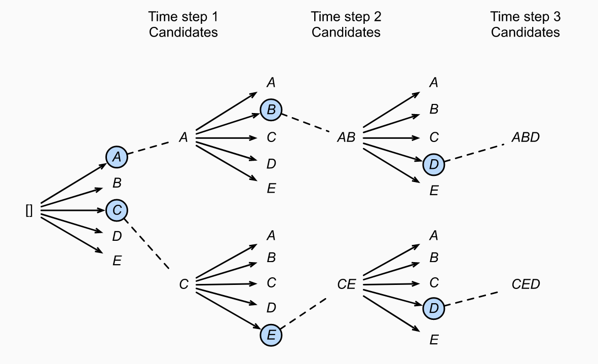
Over this full process, we have generated six candidate output sequences: $A$, $C$, $AB$, $CE$, $ABD$ and $CED$. After discarding the tails of sequences including and following <eos>, we choose the sequence which maximizes:

$\frac{1}{L^{\alpha}} \log P(y_1, \dots y_{L} \mid c) = \frac{1}{L^{\alpha}} \sum_{t' = 1}^{L} \log P(y_{t'} \mid y_1, \dots, y_{t' - 1}, c)$

where $L$ is the length of the sequence and $\alpha = 0.75$. The $L^{\alpha}$ term helps longer sequences which will have more (negative) terms in the summation.

The compute cost of beam search is $O(k \lvert \mathcal{Y} \rvert T')$. Greedy search is just beam search with $k = 1$.