CNNs

This is part 4 of my applied DL notes. They will cover very high-level intuition about CNNs.

Motivation

• Sample efficient: Take advantage of spatial structure of images, rather than igoring order of features.
• Computationally efficient: Fewer parameters then fully-connected NNs and convolutions are easier to parallelize on GPUs.

Basics

Some desirables for processing image-type sequence data:

1) Early layers should be translationally invariant.

A shift in a 2D input $X$ shoud simply lead to a shift in the hidden representation $H$. Neurons should not respond differently based on the global location of the same patch. That means we use convolutions! That is if $V$ is a weight matrix we have:

$[H]_{i, j} = u + \sum_{a} \sum_{b} [V]_{a, b} [X]_{i + a, j + b}$

Notice that $V$ does not depend on $(i, j)$, while it could. Pooling also helps with translational invariance.

2) Early layers should be capture local information.

We should not have to look far from $(i, j)$ to glean info about what is going on at $H_{i, j}$. That is for some $\Delta > 0$, we want:

$[H]_{i, j} = u + \sum_{a = -\Delta}^{\Delta} \sum_{b = -\Delta}^{\Delta} [V]_{a, b} [X]_{i + a, j + b}$

This is exactly what we call a convolutional layer. The smaller $\Delta$, the smaller the number of parameters. In general, we are going to actually have $c$ input channels (i.e. RGB images) and may want to have $d$ output channels, So:

$[H]_{i, j, d} = \sum_{a = -\Delta}^{\Delta} \sum_{b = -\Delta}^{\Delta} \sum_{c} [V]_{a, b, c, d} [X]_{i + a, j + b}$

Intuitively, one channel may be a “feature map” which learns edge detection while another learns textures.

3) Later layers should capture global information.

Since we are usually interested in global questions such as “Does this whole image contain a cat?”, we want later layers to aggregate information from earlier layers. Each hidden node should have a large receptive field with respect to the inputs. Pooling helps spatially downsample local representations.

Implementation Details

• Parameters to learn in a convolutional layer: kernel and scalar bias,
• You can increase the receptive field of an element by increasing the size of the kernel or building a deeper NN.
• Assuming an input shape of $n_{h} \times n_{w}$ and a kernel shape of $k_{h} \times k_{w}$, output shape will be $(n_{h} - k_{h} + 1) \times (n_{w} - k_{w} + 1)$ since kernel goes out of bounds.
• To avoid losing info on pixels at boundaries of images, use padding. If we add $p_{h}$ total padding rows and $p_{w}$ total padding cols, a choice which mantains dimension is $p_{h} = k_{h} - 1$ and $p_{w} = k_{w} - 1$.
• If $k_{h}$ is even, then you will have to put one more padding row on top or bottom; you will not have an even split. Using odd kernel windows is common as it ensures the output $Y_{i, j}$ comes from the cross-correlation computed with input centered at input $X_{i, j}$.
• For computational efficiency or to downsample, you can use a stride, which is the number of rows or columns traversed per slide of the kernel window. You can have a different vertical and horizontal stride. By default, they all equal 1. In general, the output shape will be $\text{floor}((n_{h} - k_{h} + p_{h} + s_{h})/s_{h}) \times \text{floor}((n_{w} - k_{w} + p_{w} + s_{w})/s_{w})$.
• If you have multiple input channels, $c_{i} > 1$, and single output channel, $c_{o} = 1$, we use a 3D kernel $c_{i} \times k_{w} \times k_{h}$. Here we do a separate 2D cross-correlation on each input channel and sum them together to get a single 2D output.
• Typically, we want more output channels as go deeper in the NN, usually downsampling to trade off spatial resolution for channel depth. To get $c_{o} > 1$ output channels, we use a 4D kernel $c_{o} \times c_{i} \times k_{w} \times k_{h}$. Here we do a separate 3D cross-correlation for each output channel and concatenate them together.
• Recall that the representations learned by channels are optimized jointly. So, it is not totally correct to say one channel is an edge detector, rather some direction in the channel space is an edge detector.
• A $1 \times 1$ convolutional layer is still useful in the multi-input and/or multi-output channels case. It no longer learns from interactions of adjacent pixels in the height/width dimensions, but it does learn from the channel dimension. One can think of it as a fully-connected layer applied at each pixel location to transform $c_{i}$ input values to $c_{o}$ output values. BUT the weights are tied across pixel location. It requires $c_{o} \times c_{i}$ weights (plus bias terms). It is used to adjust the number of channels in a NN and control model complexity.
• Pooling layers work just like convolutional layers, except the kernels are deterministic. Max and average pooling takes the max and average of elements in the window respectively. No parameters to learn here. In PyTorch, a pooling window of $(p, q)$ implements a stride of $(p, q)$.
• For pooling layers, $c_{i} = c_{o}$. Each channel is processed independently; there is no aggregation.
• While CNNs have fewer parameters, they are still expensive to compute since each parameter is involved in many more multiplications.

Architectures

Below is a summary of the history of top-performing CNNs for image classification.

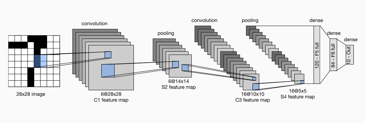
• 1998: LeNet (LeCun). It consists of two convolutional blocks (sigmoid activations + average pooling) and a dense block of three fully-connected layers. Generally, LeNet reduces spatial resolution while increasing the number of channels in the convolutional blocks.

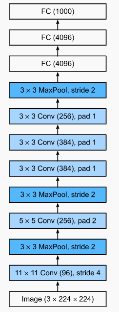
• 2012: AlexNet (Krizhevsky, Sutskever and Hinton). This architecture was inspired by the idea that we should be getting NNs to do end-to-end training. Until this point, bigger datasets or clever manually-engineered datasets meant superior performance; the details of a ML algorithm had little do with it. AlexNet emphasizes learning hierarchial representations of visual data. It was made possible by having more data and the realization we could do convolution math/linear algebra efficiently on GPUs. Below compares LeNet to AlexNet. It is obviously deeper, handles the larger ImageNet sizes, uses ReLu activations and max pooling. ReLu activations are faster to compute and avoid issues with saturation, i.e. when sigmoids are very close to 0 or 1 which slow down gradient-based learning. Finally, it also uses dropout on the dense layers (as opposed to just weight decay) and also leveraged data augmentation.

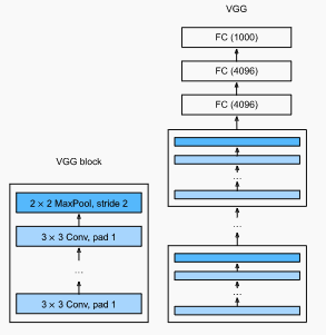
• 2014: VGG Network (Simonyan and Ziserman). This represented the shift from thinking about layers to thinking about gruops of layers, blocks. A VGG blocks is a sequence of convolutional layers (conv + ReLU) followed by a max pooling layer. The VGG network consists of: 1) five VGG blocks with increasing convolutional layers, increasing output channels and decreasing spatial resolution followed by 2) three fully-connected layers. Experimentally, they found several layers of deep and narrow convolutions ($3 \times 3$) was more effective than fewer layers of wider convolutions.

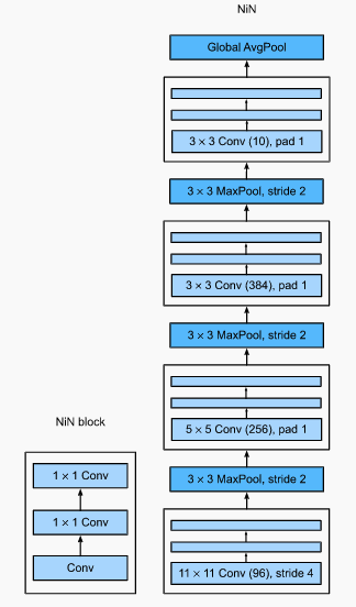
• 2013: Network in Network, NiN (Lin, Chen and Yan). What about using FC layers earlier in the network? Then, we may give up spatial structure. Instead, we can use MLPs on the channels for each pixel independently. That is we can think of each element in spatial dimension (height and width) as a sample and a channel as a feature. The NiN block is a convolutional layer followed by two $1 \times 1$ convolutional layers that function as per-pixel MLPs. One difference with AlexNet is that there are no FC layers at the end. Instead, there is a NiN block with $c_{o}$ set to the number of classes and then a global average pooling layer giving a vector of logits. Removing the FC layers reduces overfitting; NiN has way fewer parameters

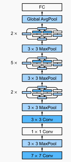
• 2014: GoogLeNet. This network combined NiN ideas with repeated blocks. A key contribution was the Inception block, a subnetwork with four paths which uses various-sized kernels to give diverse filters. The number of parameters dedicated to a given filter can also be adjusted by increasing/decreasing the numbers of output channels along each path. The final architecture starts similar to AlexNet, then stacks inception blocks and finally uses a global average pooling to avoid an FC layer stack at the end.

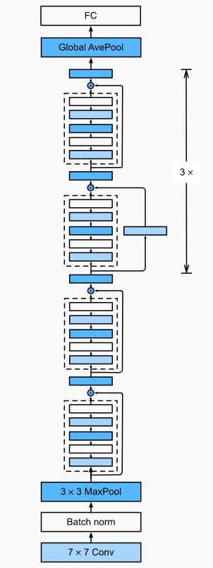
• 2016 (He, Zhang, Ren and Sun): ResNet. One would think that deeper and deeper NNs form nested function classes. This is because if I had a FC layer to a given architecture, it should be able to learn the identity function $f(x) = x$. However, empirically training deeper NNs can lead to worse training error. Optimization issues, especially vanishing/exploding gradients, are the the culprit here. ResNets facilitate layers in learning the identity function. Consider the image below. A regular block must learn the the mapping $f(x)$. A residual block needs to learn the residual mapping $f(x) - x$. If $f(x) = x$, the residual mapping is easier to learn. One just needs to set the last weight layer approximately to zero. With residual blocks, inputs can forward propogate faster. The ResNet architecture is similar to GoogLeNet, largely replacing inception blocks with residual blocks.

• 2017: DenseNet (Huang, Liu, Van Der Maaten and Weinberger). One can think of ResNet as doing a first-order Taylor approx around $x = 0$ given by $f(x) = x + f'(0)x \approx x + g(x)$, a linear plus nonlinear term. What if we want to capture info beyond the first two terms? Instead, of addition we can do concatenation and map input $x$ to an increasingly complex sequence of functions $x \rightarrow [x, f_1(x), f_2([x, f_1(x)]), \dots]$. This is exactly what DenseNet does. It consists of dense blocks, which are just a series of convolution blocks, but we concatenate the input/outputs of each block on the channel dimension. The number of channels can get unwiedly, so transition blocks are $1 \times 1$ convolution layers which control complexity and do spatial de-resolution. The final architecture is similar to ResNets.