Batch Normalization

This is part 3 of my applied DL notes. It covers a very specific topic: batch normalization.

Problems with Training NNs

As motivation, we list some common issues with training NNs that batchnorm may address:

• Performance often depends on how one chooses to process raw data. Typically, one standardizes the features to be mean 0 and std 1. Intuitively, in the case where all features matter equally, this makes optimization easier since it makes all parameters of the model on the same scale.
• Even when the original features are standardized, during the training process, the values of intermediate layers can take a wide range of magnitudes. This is true across the NN from input to output, across units of a fixed layer, and over time as model parameters change. The original authors in IS2015 informally proposed a core issue was internal covariate shift. Specifically, consider a given intermediate layer. As the parameters of preceding layers change, the distribution of inputs also changes. This forces the parameters of this layer to constantly readjust to solve a new optimization problem, making training inefficient. While not mathematically precise, one can see the means/std of inputs to layers change during the training process.
• Setting learning rates is difficult due to how strongly layers in a NN depend on the others. When we do the GD update for the weight matrix of a given layer, we implicitly assume the other layers are fixed. But we actually update all layers together. Consider a NN with no activation and single units: $\hat{y} = x w_{1} w_{2} \dots w_{l}$. Let the output of layer $i$ be given by $h_{i} = h_{i - 1} w_{i}$. Suppose that $\frac{\partial l}{d \hat{y}} = 1$, so we want to decrease $\hat{y}$ a bit. We let backprop compute $g = \left(\frac{\partial \hat{y}}{\partial w_{1}}, \dots, \frac{\partial \hat{y}}{\partial w_{l}}\right)$ and we have the GD update $w \leftarrow w - \eta g$. By a first-order Taylor approx, $\hat{y}$ decreases by $\eta g^{T}g$, so decreasing $\hat{y}$ by 0.1 would mean setting $\eta = \frac{0.1}{g^{T}g}$. But in fact, the new value of $\hat{y}$ will include second, third, $\dots$, l-order effects. The new output is $\hat{y} = x(w_{1} - \eta g_{1})(w_{2} - \eta g_{2})\dots(w_{l} - \eta g_{l})$. So, it is very difficult to choose $\eta$ because the effects of updating $w_{l}$ depend on $w_{l - 1}, \dots, w_{1}$. While second-order optimization methods may help somewhat, in truly deep NNs, even higher order interactions can matter a great deal.
• Deep NNs are at risk of overfitting and regularization is important.

Batch Normalization Overview

Batchnorm addresses some of these issues and consistently helps accelerate convergence of deep NNs (sometimes with depth > 100). Batchnorm is applied layer-by-layer. In each training iteration, the inputs are standardized based on the estimated mean/std of the current minibatch and then scaled based on a learned scale coefficient/offset. More precisely, for minibatch $\mathcal{B}$ and input $x \in \mathcal{B}$ to a batchnorm operation, we have:

$\text{BN}(x) = \beta \odot \frac{x - \hat{\mu}_{\mathcal{B}}}{\hat{\sigma}_{\mathcal{B}}} + \alpha$

where $\hat{\mu}_{\mathcal{B}}$ is the sample mean and $\hat{\sigma}_{\mathcal{B}}$ is the sample std of minibatch $\mathcal{B}$, calculated per dimension. Standardizing to mean 0 and std 1 is potentially an arbitrary choice and can reduce the expressive power of the NN. Hence we include scale parameters $\beta$ and $\alpha$, which are learned jointly with the rest of the model parameters and are of the same size as the input $x$. Note we usually add some small constant $\epsilon$ to $\hat{\sigma}_{\mathcal{B}}$ in order to prevent divide by zero errors.

For batchnorm to work we need minibatches of size greater than 1; that is $\lvert \mathcal{B} \rvert > 1$. Otherwise, each hidden unit would take a value of 0. Batchnorm tends to work effectively for standard minibatch sizes. However, the key point is that the use of batchnorm makes one’s choice of minibatch size even more important.

For batchnorm to work in practice, we just add batchnorm layers to the NN. It is a differentiable operation and the gradient of the loss with respect to the different parameters can be computed with the chain rule as usual. However, unlike other operations, the minibatch size will show up in the gradient formulas. Consider fully-connected layers. Denote the input as $x$, the weight matrix as $W$, the bias vector as $b$ and activation as $\phi$. The output, $h$, is then given by:

$h = \phi(\text{BN}(Wx + b))$

In certain applications, you can also put the $\text{BN}$ operation after the activation $\phi$. Convolutional layers will be a little different. We can apply $\text{BN}$ after convolution and before $\phi$. If there are multiple output channels, batchnorm is applied to each channel and each channel has its own scale coefficient/offsets, which are scalars. Assume that $\lvert \mathcal{B} \rvert = m$ and the convolution output has height $p$ and width $q$. Then, per output channel, batchnorm will compute the mean/std over $m \times p \times q$ elements.

Another detail to keep in mind is how batchnorm works differently during train and inference times. In train time, the variable values are standardized by minibatch statistics. It would be impossible to use the full dataset statistics because the variable values change every time a minibatch passes through and model parameters are updated. In the inference stage, we have a fixed trained model and can use full dataset statistics to get estimates with less sample noise. Moreover, in the inference stage, we may be making predictions one at a time, so do not even have access to the original minibatches. In practice, people keep track of EWMAs of the intermediate layer sample means/stds and use these statistics for inference. In PyTorch, you typically want to set the momentum parameter to 0.1 or 0.01, which correspond to the weight on the latest minibatch statistic. The closer we set momentum to 0, the more we are relying on historical minibatches.

Why Does It Help?

In some sense, batchnorm does not seem to do anything because it standardizes variable values with $\hat{\mu}_{\mathcal{B}}$ and $\hat{\sigma}_{\mathcal{B}}$, but then scales them back with $\alpha$ and $\beta$. The key idea is that parameterizing NNs with and without batchnorm can represent the same set of functions, but using batchnorm makes optimization with standard algorithms like GD is much easier. Empirically, DL practitioners have found that batchnorm allows for more aggressive learning rates without vanishing/exploding gradients (so faster convergence) and makes training a NN robust to different initializations and/or learning rates. Intuitively, it seems to play the same role as pre-standardizing one’s features in non-deep ML. Moreover, inputs to intermediate layers cannot diverge to crazy magnitudes during training since they are actively re-standardized. Moreover, for particular activation functions $\phi$, it may help keep variable values in the non-saturating regime. For linear 1-layer NNs, one can explicitly show that batchnorm implies a better conditioned Hessian.

Going back to our example $\hat{y} = x w_{1} w_{2} \dots w_{l}$, we can see more precisely how batchnorm solves the stated issues and makes learning easier. Specifically, assume that $x$ is $\mathcal{N}(0, 1)$. Then it is clear that $h_{l - 1}$ will also be Gaussian, but not with mean 0 and std 1. However, $\text{BN}(h_{l - 1})$ is back to being $\mathcal{N}(0, 1)$ and will remain so for almost any update to lower layers. Hence we can learn the simple linear function $\hat{y} = w_{l} \text{BN}(h_{l - 1})$. Since the parameters from the preceding layers do not have any effect anymore, learning here is a simple task. There are corner cases where lower layers do have an effect. For example, if one changes $w_{i \leq l - 1}$ to 0, the output is degenerate. Also, if one flips the sign of $w_{i \leq l - 1}$, then the relationship between $\text{BN}(h_{l - 1})$ and $y$ also flips sign. In this example, we have stabilized learning at the expense of making the earlier layers useless. But this is because we have a linear model. With non-linear activations, the preceding layers remain useful.

In addition to improving training, batchnorm improves generalization. One theory is that batchnorm has a regularization effect. Empirically, practitioners have found that dropout tends to be less important when using batchnorm. First, the use of minibatches adds a source of noise to the training process (much like dropout) which for unknown reasons causes less overfitting. More precisely, since the samples in a given minibatch are randomly selected, the quantities $\hat{\mu}_{\mathcal{B}}$ and $\hat{\sigma}_{\mathcal{B}}$ introduce random fluctuations to the training process of hidden layers. More theoretically, the authors in LWSP18 analyze batchnorm in a Bayesian framework. They connect its effect to imposing particular priors/penalities on parameters which encourage the NN to not over-rely on a particular neuron and reduce correlations among different neurons. In this set-up, the strength of regularization is inversely proportional to $\lvert \mathcal{B} \rvert$, indicating that making the minibatch too large may not be optimal. This result is consistent with the finding that batchnorm works best for minibatches of sizes 50-100.

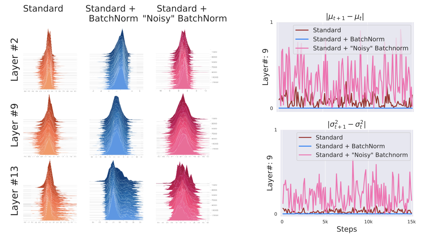
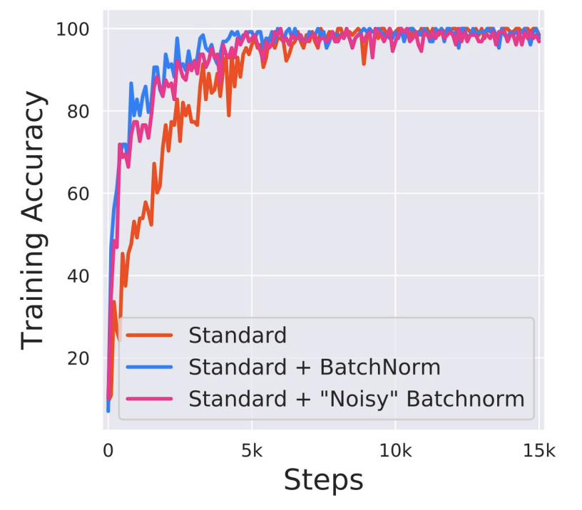
The theoretical backing for batchnorm’s optimization improvement is controversial. In STIM18, the authors argue it has nothing to do with internal covariate shift. They look at histograms of the inputs into a various layers and find that these histograms are fairly stable over the course of training iterations for both standard and batch normalized VGG NNs. The authors then create a “noisy” batchnorm NN where they add non-stationary Gaussian noise to the outputs of the batchnorm layer. While the histograms of this “noisy” batchnorm are noticeably less stable, it still converges faster than a standard NN.

Instead, the authors argue that batchnorm has a smoothing effect on the optimization landscape which makes first-order methods more quicker and more robust to hyperparameter choices. They measure the variation of the value of the loss, $\mathcal{L}(x - \eta \nabla \mathcal{L}(x))$, and change of the loss gradient, $\|\nabla \mathcal{L}(x) - \nabla \mathcal{L}(x - \eta \nabla \mathcal{L}(x))\|$ for $\eta \in [0.05, 0.4]$ over the course of training. They find that the batchnorm network has smaller variability of loss and smaller change of the loss gradient. So, steps taken during GD are unlikely to drive the loss very high and the gradient at a point $x$ stays relevant over longer distances supporting larger $\eta$. More precisely, their theoretical analysis shows batchnorm improves the Lipschitzness of both the loss and gradients (i.e. $\beta$-smoothness). Together these imply that the gradients are more predictive allowing for larger learning rates and faster convergence.

The theory of batchnorm is again brought into question by CKLKT21. The authors argue that for a wide range of practical learning rates and many NN architectures, full-batch GD very quickly enters the edge of stability:

• The local smoothess, i.e. the max eigenvalue of the training loss Hessian, hovers right at or above $2/\eta$. In such a regime, GD would not work for convex objectives.
• The loss behaves non-monotonically but decreases over long time scales.

They find this phenomenon holds for both standard and batch normalized VGG NNs. Hence they state that the experiments in STIM18 cannot be interpreted as showing that batchnorm improves the local smoothness of the loss along the optimization trajectory. Some of the empirical analysis here is based on re-doing the experiments with a more appropriate measure for “effective smoothness” and showing that this new measure does not actually show better behavior in the batchnorm setting.