Deep Learning Basics

I plan on putting together some personal applied deep learning notes. They will pull together:

• More practical advice from these two textbooks, ZLLS2021 and GBC2016
• Other insights from my courses, notes available online and papers

The following post will start with DL basics.

Automatic Differentiation

Autodiff is a general framework to compute derivatives, not just of mathematical functions, but general programs with control flow. Standard techniques for evaluating derivatives have disadvantages:

• Manual calculus: not scalable, painful for complex functions
• Symbolic (à la Maple): expressions explode, only applicable to closed form functions
• Numerical: For a function $f: \mathbb{R}^d \rightarrow \mathbb{R}$ need to run $d$ approximation times, unstable, depends on choice of $h$ when computing $f'(x) \approx \frac{f(x + h) - f(x)}{h}$

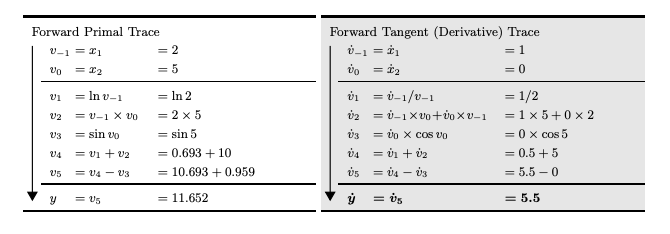
Autodiff is a symbolic/numerical hybrid. The core idea is that all algorithms can be written as a composition of simple functions with known derivatives. This is called the trace and can be represented as a DAG. Consider the example from BPRS2015 where $f(x_1, x_2) = \log(x_1) + x_1x_2 - \sin(x_2)$. To evaluate derivatives, we do the following:

• Break down $f$ into its trace: $v_{-1} = x_1$, $v_1 = \log(v_{-1})$, $\dots$
• Compute symbolic derivatives for each op in the trace: $\dot{v}_{-1} = \frac{\partial v_{-1}}{\partial x_1} = 1$, $\dot{v}_1 = \frac{\partial v_{1}}{\partial x_1} = \frac{\dot{v}_{-1}}{v_{-1}}$, $\dots$
• Apply the chain rule: Recurse through the trace and numerically compute the exact derivatives

Any control flow code is just eliminated: branches are taken, loops unrolled, etc. This leaves us with a linear execution trace. The above formulation is known as forward mode autodiff. It is efficient for functions $g: \mathbb{R}^N \rightarrow \mathbb{R}^M$ where $N \ll M$. It will require just $N$ passes to compute the Jacobian. It provides matrix-free way of for evaluating Jacobian-vector products. Specifically:

$J_{f} r = \begin{bmatrix} \frac{\partial y_1}{\partial x_1} & \dots & \frac{\partial y_1}{\partial x_n}\\ \dots & \dots & \dots \\ \frac{\partial y_m}{\partial x_1} & \dots & \frac{\partial y_m}{\partial x_n}\\ \end{bmatrix} \begin{bmatrix} r_1\\ \dots\\ r_n \end{bmatrix}$

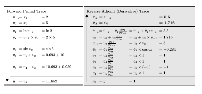
can be computed in a single forward pass by initializing $\dot{x} = r$. For functions where $N \gg M$, like neural nets, we use reverse mode autodiff. Here the derivatives are propogated back from a given output. Again, consider our example and let $y = f(x_1, x_2)$. If we define $\bar{v}_i = \frac{\partial y}{\partial v_{i}}$, then we see the total derivative with respect to $v_0$ is:

$\bar{v}_0 = \bar{v}_2 \frac{\partial v_2}{\partial v_0} + \bar{v}_3 \frac{\partial v_3}{\partial v_0}$

We can compute such values in a two step procedure. First, run a forward pass to compute the intermediate values of $v_i$ and track the dependencies in the DAG. Second, propogate the derivatives backward from outputs to inputs.

This process will require $M$ passes to compute the Jacobian of $g$. Reverse mode provides a matrix-free way of computing transposed Jacobian-vector products. Specifically:

$J^{T}_f r = \begin{bmatrix} \frac{\partial y_1}{\partial x_1} & \dots & \frac{\partial y_m}{\partial x_1}\\ \dots & \dots & \dots \\ \frac{\partial y_1}{\partial x_n} & \dots & \frac{\partial y_m}{\partial x_n}\\ \end{bmatrix} \begin{bmatrix} r_1\\ \dots\\ r_m \end{bmatrix}$

can be computed in a single forward + backward pass by initializing $\bar{y} = r$. Note that when $M = 1$, that means we can get the gradient $\nabla_{x} f(x)$ in a single pass.

The Python package autograd wraps numpy ops to support autodiff. Reverse mode autodiff is also what is going on when you do x.backward() in PyTorch.

Backpropagation

As an example of how NNs use reverse autodiff, consider a one-hidden layer MLP with $L_2$ weight regularization. For simplicity, assume there are no bias terms, so all the trainable parameters are $W = (W^{(1)}, W^{(2)})$ where $W^{(1)} \in \mathbb{R}^{h \times d}$ and $W^{(2)} \in \mathbb{R}^{q \times h}$.

First, in the forward pass we take an input example $x \in \mathbb{R}^d$ and compute the following:

$o = W^{(2)}h = W^{(2)}\phi(z) = W^{(2)}\phi(W^{(1)}x)$

The objective function for that example is computed as:

$J(x, y) = L(o, y) + s(W)$

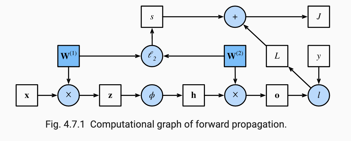
where $L(o, y)$ might be cross-entropy loss and $s(W) = \frac{\lambda}{2}\left(\|W^{1}\|_{F}^2 + \|W^{2}\|_{F}^2\right)$. The following image from ZLLS2021 shows the DAG associated with this NN:

Second, in the backward pass, we start with the following:

$\frac{\partial J}{\partial L} = 1 \quad \quad \frac{\partial J}{\partial s} = 1$

Then, we compute the gradient of the $J$ with respect to outputs $o$:

$\frac{\partial J}{\partial o} = \text{prod}\left(\frac{\partial J}{\partial L}, \frac{\partial L}{\partial o}\right) = \frac{\partial L}{\partial o} \in \mathbb{R}^q$

Next, we compute the gradient of the regularization with respect to $W$:

$\frac{\partial s}{\partial W^{(1)}} = \lambda W^{(1)} \quad \quad \frac{\partial s}{\partial W^{(2)}} = \lambda W^{(2)}$

Then, we can compute the gradient for $W^{(2)}$:

$\frac{\partial J}{\partial W^{(2)}} = \text{prod}\left(\frac{\partial J}{\partial o}, \frac{\partial o}{\partial W^{(2)}}\right) + \text{prod}\left(\frac{\partial J}{\partial s}, \frac{\partial s}{\partial W^{(2)}}\right) = \frac{\partial J}{\partial o}h^{T} + \lambda W^{(2)} \in \mathbb{R}^{q \times h}$

For the gradient of $W^{(1)}$, we need to continue:

$\frac{\partial J}{\partial h} = \text{prod}\left(\frac{\partial J}{\partial o}, \frac{\partial o}{\partial h}\right) = (W^{(2)})^{T}\frac{\partial J}{\partial o}$

$\frac{\partial J}{\partial z} = \text{prod}\left(\frac{\partial J}{\partial h}, \frac{\partial h}{\partial z}\right) = \frac{\partial J}{\partial h} \circledcirc \phi^{'}(z)$

where $\circledcirc$ is the element wise multiplication operator. Finally, we get:

$\frac{\partial J}{\partial W^{(1)}} = \text{prod}\left(\frac{\partial J}{\partial z}, \frac{\partial z}{\partial W^{(1)}}\right) + \text{prod}\left(\frac{\partial J}{\partial s}, \frac{\partial s}{\partial W^{(1)}}\right) = \frac{\partial J}{\partial z}x^{T} + \lambda W^{(1)} \in \mathbb{R}^{h \times d}$

The above steps are computationally efficient compared to forward mode autodiff in two ways:

• First, when computing $\frac{\partial J}{\partial W^{(1)}}$ we were able to avoid duplicate re-computations of the component of the gradient associated with the hidden layer and beyond. Thinking about a NN as a graph, forward mode is $\Theta(V^2)$ while reverse mode is $O(E)$.
• Second, note that $\frac{\partial J}{\partial o}$ was a vector in $\mathbb{R}^q$. Computing $\frac{\partial J}{\partial W^{(1)}}$ only required matrix-vector products. Forward mode tracks how changes in $W^{(1)}$ pass through to $o$ and would require matrix-matrix products since $W^{(2)}$ is in between. So, reverse mode takes advantage of the fact that we only care about how weight changes affect the final loss to reduce the number of matrix-matrix computations.

The downside of reverse mode autodiff is memory complexity. It requires storage of all intermediate quantities from the forward pass to compute gradients. Memory requirements scale proportionally to the number of layers and batch size. So, training deep networks with large batches can lead to out of memory errors. That is with backward mode we pay $O(V)$ is memory cost.

Softmax Operation

For classification, we need to transform real-valued logits $o$ to a discrete probability distribution $\hat{y}$. The softmax operation does this transformation in a way that makes it differentiable, ensures $\sum_{i} \hat{y}_j = 1$ and $\hat{y}_j > 0$. Specifically, we have:

$\hat{y} = \text{softmax}(o) \quad \text{where} \quad \hat{y}_j = \frac{\exp(o_j)}{\sum_{k} \exp(o_k)}$

Cross-Entropy Loss

Say we have $q$ classes. Minimizing cross-entropy loss is equivalent to minimizing the negative log likelihood of our data where we assume that $P(y^{(i)} \mid x^{(i)}) = \text{Multinomial}(n = 1, p = \hat{y}_i)$. We have:

$-\log P(Y \mid X) = -\sum_{i = 1}^n \log P(y^{(i)} \mid x^{(i)}) = -\sum_{i=1}^n l(y^{(i)}, \hat{y}^{(i)}) = -\sum_{i=1}^n \sum_{j = 1}^q y^{(i)}_j \log \hat{y}^{(i)}_j$

Note that $\log \hat{y}^{(i)}_j = 0$ if $\hat{y}^{(i)}_j = 1$; that is we predict class $j$ with perfect certainty. Else, $\log \hat{y}^{(i)}_k < 0$. We have:

$\begin{aligned} l(y, \hat{y}) &= -\sum_{k = 1}^q y_k \log \frac{\exp(o_j)}{\sum_{k} \exp(o_k)}\\ &= \log \sum_{k = 1}^q \exp(o_k) - \sum_{j = 1}^q y_j o_j \end{aligned}$

The derivative with respect to a logit $o_j$ becomes:

$\partial l_{o_j}(y, \hat{y}) = \frac{\exp(o_j)}{\sum_{k = 1}^q \exp(o_k)} - y_j = \text{softmax}(o)_j - y_j$

This result is similar to OLS where the gradients of square loss are of the form $\hat{y} - y$. The gradients of any EFM model are of this form, making them trivial to compute. All of this math holds even when our label $y$ is not a binary vector but a distribution of the form $y = (0.1, 0, 0.4, 0.5)$. In that case, we can think of cross-entropy in information-theoretic terms. We are minimizing:

$H(P_{y}, P_{\hat{y}}) = H(P_{y}) + D_{\text{KL}}(P_{y} \mid \mid P_{\hat{y}})$

with $D_{\text{KL}}(P_{y} \mid \mid P_{\hat{y}}) = 0$ if $P_{y} = P_{\hat{y}}$ and $>0$ otherwise.

Handling Numerical Issues with Softmax

If some of the logits $o_k$ are very large, then $\exp(o_k)$ might be larger than the largest number than can be handled by certain data types. A simple solution is to subtract $\max(o_k)$ from all the logits. This does not change the softmax outputs:

$\begin{aligned} \hat{y}_j &= \frac{\exp(o_j - \max(o_k))\exp(\max(o_k))}{\sum_{k} \exp(o_k - max(o_k))\exp(\max(o_k))}\\ &= \frac{\exp(o_j - \max(o_k))}{\sum_{k} \exp(o_k - max(o_k))} \end{aligned}$

Now we face another issue: $o_j - \max(o_k)$ might be very negative and $\exp(o_j - \max(o_k))$ might be close to 0. Due to finite precision, these values may be rounded to 0. And then we will have $\log(-\hat{y_j}) = -\text{inf}$. However, recall that ultimately we plug in the softmax outputs into cross-entropy loss where we take a log. Hence we get:

$\log \hat{y}_j = o_j - \log \left(\sum_{k} \exp(o_k) \right)$

Hence we can avoid computing $\exp(o_j - \max(o_k))$ by directly computing $\log \hat{y}_j$ in the cross-entropy loss function. Finally, we can take advantage of the LogSumExp trick:

$\log\left(\sum_{k} \exp(o_k) \right) = \max(o_k) + \log \left(\sum_{j} \exp(o_j - \max(o_k))\right)$

These tricks are implemented in torch.nn.CrossEntropyLoss().

Multilayer Perceptrons

A $L$-layer MLP is given by:

$O = \sigma_{L-1}(\dots \sigma_2(\sigma_1(XW^{(1)} + b^{(1)})W^{(2)} + b^{(2)}) \dots)W^{L} + b^{L}$

where $\sigma_i$ are activation functions which usually operate element or row wise and $W^{(i)}$ and $b^{(i)}$ are the trainable model weights and biases. Note that it is key that $\sigma_i$ are non-linear. Otherwise, we are just building a a single-layer linear model with more parameters than necessary.

MLPs are known as universal approximators. Several different statements exist formalizing this intuition. One is that three-layer MLPs can approximate any $L$-Lipschitz function $f: [0, 1]^d \rightarrow \mathbb{R}$ with $O\left(d\left(\frac{L}{\epsilon}\right)^d\right)$ neurons and ReLU activations such that $L_1$ error is bounded by $\epsilon$:

$\int_{[0, 1]^d} \left\lvert f(x) - \hat{f}(x) \right\rvert dx \leq \epsilon$

Finding such a $\hat{f}$ in a computationally efficient manner is the hard part. Also, not the exponential dependence on dimension $d$ here.

Activation Functions

• ReLU: $\sigma(x) = \max(0, x)$. ReLU is common because the derivatives are well-behaved. They vanish when $x \leq 0$ or equal one when $x > 0$. This makes optimization easier and mitigates issues with vanishing gradients.

• Parametrized ReLU: $\sigma(x) = \max(0, x) + \alpha \min(0, x)$. Some information gets through even when $x < 0$.

• Sigmoid: $\sigma(x) = \frac{1}{1 + \exp(-x)}$. Maps inputs $x$ to $(0, 1)$. We have $\sigma'(x) = \sigma(x)(1 - \sigma(x))$. Hence $\sigma'(x) \rightarrow 0$ as $x \rightarrow \infty$ or $x \rightarrow -\infty$. Small gradients for very small or very large $x$ can lead to slow updated during GD.

• Tanh: $\sigma(x) = \frac{1 - \exp(-2x)}{1 + \exp(-2x)}$. Maps inputs $x$ to $(-1, 1)$ and exhibits point symmetry around the origin. We have $\sigma'(x) = 1 - \sigma(x)^2$. Hence $\sigma'(x) \rightarrow 0$ as $x \rightarrow \infty$ or $x \rightarrow -\infty$. Sometimes preferable to sigmoid for hidden layers because mean of output tends to be close to 0, centering the data for future layers.

Regularization

Weight Decay

Similar to high-dimensional linear regression, a common strategy to regularize is to add $L_2$ or $L_1$ penalties on the weight matrices $W^{(i)}$ to force the model to fit smoother functions. Whether the bias terms are penalized varies across applications, but usually it is not penalized in the output layer. For simplicity, assume all the weight matrices are vectorized are represented by parameter $w$. The new regularized loss is of the form:

$L_{R}(w, b) = \frac{\lambda}{2} w^{T}w + L(w, b)$

The GD steps look like:

$w \leftarrow (1 - \eta\lambda) w - \eta \nabla_{w} L(w, b)$

So, the weights are shrunk by a constant factor each step before perfoming the standard GD update. We can also study what happens over the course of the full training procedure. Let $w^{\ast} = \arg\min L(w, b)$, the unregularized loss. Then, by a second order Taylor approximation around $w^{\ast}$:

$\hat{L}_{R}(w, b) = L_{R}(w^{\ast}, b) + \lambda (w^{\ast})^{T}(w - w^{\ast}) + \frac{1}{2}(w - w^{\ast})^{T}H(w - w^{\ast}) + \lambda$

where $H$ is the hessian of $L(w, b)$ at $w^{\ast}$. Since $w^{\ast}$ is the minimizer, it is PSD. Note part of the first order term disappears because $\left[\nabla_{w} L(w, b)\right]_{w = w^{\ast}} = 0$. The minimum of $\hat{L}_{R}(w, b)$ occurs when $\nabla_{w} \hat{L}_{R}(w, b) = \lambda w + H(w - w^{\ast}) = 0$:

$\hat{w} = (H + \lambda I)^{-1}Hw^{\ast}$

Note as $\lambda \rightarrow 0$, we have $\hat{w} \rightarrow w^{\ast}$. Else taking the eigendecomposition $H = Q\Delta Q^{T}$:

$\hat{w} = Q(\Delta + \lambda I)^{-1}\Delta Q^{T} w^{\ast} \tag{1}$

This is exactly the same analysis as ridge regression. We see that weight decay aligns the components of $w^{\ast}$ that are aligned with the $i$-th eigenvector of $H$ are scaled by $\frac{\gamma_i}{\gamma_i + \lambda}$ where $\gamma_i$ are the eigenvalues. Directions in the parameter space which do not contribute much to reducing $L(w, b)$ and hence have small eigenvalues are significantly shrunk by $L_2$ weight decay.

We can similarly do $L_1$ regularization. Then, we have:

$L_{R}(w, b) = \lambda \|w\|_{1} + L(w, b)$

The GD updates look like:

$w \rightarrow w - \lambda \text{sign}(w) - \eta \nabla L_{w}(w, b)$

where $\text{sign}(w)$ is applied component-wise. If we assume the Hessian is diagonal:

$\hat{L}_{R}(w, b) = L_{R}(w^{\ast}, b) + \sum_{i} \left[\frac{1}{2}H_{i, i}(w_i - w^{\ast}_i)^2 + \lambda \lvert w_i \rvert \right]$

The component-wise solution is given by:

$\hat{w_i} = \text{sign}(w_i^{\ast})\max\left\{\lvert w_i^{\ast} \rvert - \frac{\alpha}{H_{i, i}}, 0\right\}$

Again, this is exactly the same as the Lasso analysis. The thresholding operation will encourage shrinkage plus sparsity.

In PyTorch, $L_2$ penalization is automatically supported with by adding weight_decay=lambda as an argument to torch.optim.SGD(). You have to define a custom loss functionf or $L_1$ penalization.

Early Stopping

Early stopping refers to terminating training when you start to see validation error trend upward over some number of past epochs. You return model parameters from the last kink you saw in the risk curve. Such a strategy can be viewed as an efficient algorithm for hyperparameter search. The hyperparameter here is the number of training steps. Unlike grid search, a single training run automatically evaluates the loss for several values of this hyperparameter. Also, it is completely unobtrusive, not changing the loss function and learning dynamics. The extra cost comes from evaluating on the validation set in each step and having to store the optimal model parameters.

Say we restrict the number of optimization steps to $\tau$ and assume that the gradient of the loss is bounded by $B$. Then, early stopping restricts $\|w_{o} - w\|_{2} \leq \eta \tau B$ where $w_{o}$ is the initialization. For more intuition, lets analyze a linear model with square loss and optimal $w^{\ast}$. We will show that early stopping is equal to $L_2$ regularization. We have:

$L(w) = L(w^{\ast}) + \frac{1}{2}(w - w^{\ast})^{T}H(w - w^{\ast})$

The GD iterates:

$w^t = w^{t - 1} - \eta H(w^{t - 1} - w^{\ast}) \Longrightarrow w^{t} - w^{\ast} = (I - \eta H)(w^{t - 1} - w^{\ast})$

Using the eigendecomposition $H = Q \Delta Q^{T}$:

$Q^{T}(w^{t} - w^{\ast}) = (I - \eta \Delta)Q^{T}(w^{t - 1} - w^{\ast})$

If $\eta$ is chosen such that $\lvert 1 - \eta \gamma_i \rvert < 1$ and $w^{0} = 0$, then we have:

$Q^{T}w^{t} = \left[I - (I - \eta \Delta)^{t}\right]Q^{T}w^{\ast} \tag{2}$

Recall from Equation $1$, we have for the $L_2$ regularization:

$Q^{T}\hat{w} = (\Delta + \lambda I)^{-1} \Delta Q^{T}w^{\ast} \Longrightarrow Q^{T}\hat{w} = [I - (\Delta + \lambda I)^{-1} \lambda]Q^{T}w$

The equality here follows from the Woodbury matrix identity. Compared to Equation $2$, they are equivalent when $\lambda$, $\eta$ and $t$ are chosen such that:

$(I - \eta \Delta)^{t} = (\Delta + \lambda I)^{-1} \lambda$

If the eigenvalues $\gamma_i$ are sufficiently small, one can show that this equivalence corresponds to $t = \frac{1}{\eta \lambda}$. That is the number of training iterations is inversely proportional to the $L_2$ parameter $\lambda$. In context of early stopping, we see that parameter directions with signifcant curvature learn early compared to directions of less curvature.

Dataset Augmentation

More training samples can improve generalization. If we do not have that, we can create fake data and add it to the training data. In computer vision, add samples with rotations or where a few pixels have been translated can force the NN to be invariant to these transformations. Make sure to not rotate a “9” to a “6” if you are asking your model to classify digits. Adding noise to your inputs can be shown in many cases to be equivalent to adding a weight norm penalty. For a proof, look at B1995.

Adding Noise to Weights

We can also add noise to the parameters of a model. Say for each input sample, we include a pertubation $\epsilon_{W} \sim N(0, \eta I)$ on the network weights. If we are using squared loss, we want to minimize the risk:

$\mathbb{E}_{p(x, y, \epsilon_{W})} \left[(\hat{y}_{\epsilon_W}(x) - y)^2 \right] = \mathbb{E}_{p(x, y, \epsilon_{W})}\left[\hat{y}_{\epsilon_W}(x)^2 - 2y\hat{y}_{\epsilon_W}(x) + y^2\right]$

For sufficiently small $\eta$, this can be shown to be the same as minimizing the unperturbated risk with a regularization term $\eta \mathbb{E}_{p(x, y)}\left[\|\nabla_{W} \hat{y}(x) \|_{2}^2 \right]$. So, the solution is pushed to regions in the parameter space where perturbations in the weights have a small effect on the predictions. We find minima surrounded by flat regions. Note that this only works for non-linear models. In linear regression, the regularization term becomes $\eta \mathbb{E}_{p(x)}\left[\|x \|_{2}^2 \right]$, which does not depend on parameters $W$.

Dropout

Dropout is a technique developed in SKHSS2014. The idea is to inject noise to the hidden units of a NN. Throughout the training process, during forward propogation, some fraction of neurons in a layer are randomly zeroed out before computing the subsequent layer. The original authors proposed a slightly different interpretation. They argued that overfitting in NNs is characterized by co-adaptation where each layer relies on a specific pattern activations in the previous layer to fit the data well. Dropout forces neurons to learn more robust features since they cannot rely on other units to correct its mistakes.

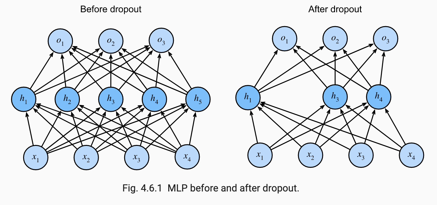
The image below from ZLLS2021 shows how dropout amounts to training a smaller sub-network of the original NN:

This provides an interpretation of dropout as an approximation to bagging. Specifically, consider the exponential number of sub-networks that can be formed by masking certain neurons in a NN. In dropout, for each training example in a mini batch, a different sub-network is sampled and then we run the forward pass, backprop and parameter update. If $\mu$ corresponds to the mask vector, dropout training can be viewed as minimizing $\mathbb{E}_{\mu}[L(w, b, \mu)]$. We can get an unbiased estimate the gradient of this function by sampling values of $\mu$. Unlike bagging, the base learners share their parameters and are not trained to convergence. Parameter sharing makes it possible to “ensemble” exponentially many sub-networks in a memory-efficient manner. Much like bagging, each sub-network sees a subset of the original training examples sampled with replacement due to minibatches.

The noise added during dropout should be added in an unbiased manner. The expected value of a layer holding all other layers fixed should be equal its value in the absence of noise. Hence an activation function $h$ is replaced with random variable $h^{'}$:

$h^{'} = \begin{cases} 0 &\quad \text{with prob } p,\\ \frac{h}{1 - p} &\quad \text{ with prob } 1- p \end{cases}$

where $p$ is the dropout probability. Notice that $\mathbb{E}[h^{'}] = h$. Since dropout is disabled at test time, this scaling ensures the expected total input to a neuron at test time is the same as the expected total input to a neuron at train time.

In practice, implementing dropout during training is as simple as drawing random uniforms and multiplying a hidden layer by mask to convert $h \rightarrow h^{'}$. Usually, the input layer has $p \approx 0$ because we do not want to turn off too many of the input features.

Adding dropout in PyTorch is as easy as using the torch.nn.Dropout class in your NN specification.

Vanishing and Exploding Gradients

Consider a NN with $L$ layers, input $x$ and output $o$ where each layer $l$ is a transformation $f_{l}$ parameterized by matrix $W^{(l)}$. Let $h^{(0)} = x$, then we have:

$h^{(l)} = f_{l}(h^{(l-1)}) \quad \quad o = f_{L}(f_{L - 1}( \dots f_1(x)))$

We can write the gradient $o$ with respect to $W^{l}$ as follows:

$\partial_{W^{(l)}}(o) = \partial_{h^{(L-1)}} h^{(L)} \cdots \partial_{h^{(l)}} h^{(l + 1)} \partial_{W^{(l)}} h^{(l)} = M^{(L)} \cdots M^{(l + 1)} v^{(l)}$

The gradient is the product of matrices and a vector. Depending on the eigenspectrum of these submatrices the gradient can end up being very small or very large. For simplicity, assume that $M = M^{(L)} = \dots = M^{(l + 1)}$ and $M$ has eigendecomposition $V \Delta V^{-1}$. Then, we have:

$\partial_{W^{(l)}}(o) = M^{(L - 1)}v^{(l)} = V \Delta^{L - 1}V^{-1}v^{(l)}$

Hence, for deep NNs, if the eigenvalues are larger than $1$ in magnitude, the gradient explodes. If the eigenvalues are smaller than $1$ is magnitude, the gradient vanishes. Exploding gradients make learning unstable. Vanishing gradients make it impossible to figure out where to move in parameter space. This problem is pronounced in RNNs where we are using the same weight matrix $M$ over and over again in many layers, but can also show up elsewhere.

One source of vanishing gradients is the choice of activation function. For example, consider the sigmoid activation. Since $\sigma^{'}(x) \approx 0$ when $x \not\approx 0$ and $\max_{x} \sigma^{'}(x) = 1/4$, if you have small weights multiplied by these activation gradients, the loss gradient can approach zero at rate exponential in the number of layers during backprop. Early layers train very slowly. ReLU solves this problem.

Exploding gradients are driven by large weights. It is more of a problem with ReLUs compared to squashing functions like the sigmoid and tanh. But for all activations, sufficiently large weights can cause the loss gradient to explode at an exponential rate. As an example, consider the following 3-layer NN where each layer has a single neuron:

$y = \tanh(w_3 \cdot \tanh(w_2 \cdot \tanh(w_1 \cdot x)))$

Then the gradient with respect to the first weight $w_1$ is:

$\begin{aligned} \frac{\partial L}{d w_{1}} = \frac{\partial L}{\partial y} \cdot w_3 \cdot w_2 \cdot x \cdot \text{sech}^2(w_1 \cdot x) \cdot \text{sech}^2(w_2 \cdot \tanh(w_1 \cdot x))\cdot \text{sech}^2(w_3 \cdot \tanh(w_2 \cdot \tanh(w_1 \cdot x))) \end{aligned}$

Note that $\text{sech}^{2}(x) \leq 1$. But for a large number of layers $L$ the term $\prod_{i = 2}^{L} w_i$ can blow up when $L$ is large and $\lvert w_i \rvert > 1$. Similar behavior is possible for the sigmoid activation.

Weight Initialization

Recall that weight initialization is not an issue for convex problems such as linear or softmax regression since the appropriate optimization algorithms are guaranteed to reach a global minimum. For non-convex problems, initialization affects the solution to which you converge and the numerical stability of the algorithm.

Breaking Symmetry

Fully connected NNs are symmetric in their parametrization. Imagine a simple MLP with one hidden layer and two units. We can permute the weights in $W^{(1)}$ and $W^{(2)}$ and obtain the exact same function. Hence there is permutation symmetry among the hidden units of each layer.

Such symmetry can become a problem during training. If the hidden units of a layer share the same input/output weights and activations, they compute the same values and receive the same gradient during backprop. The GD updates for each unit’s weights will the same. So, the hidden layer would behave as a single unit, wasting the NN’s capacity.

To break symmetry, we need to add specific forms of randomness to the training process. For a single hidden layer MLP, we will see the undesired behavior if we initialize $W^{(1)} = c$ for some constant $c$. Randomly initializing the elements in $W^{(1)}$ to small values from a Gaussian or uniform is the standard strategy. Technically, one can continue to initialize the weights into the output units, $W^{(2)} = c$. The output units receive different gradients during backprop based on the functional form of the loss. But if you start with $W^{(2)} = 0$, it will take two iterations to make $\frac{\partial L}{\partial W^{(1)}} \neq 0$ and finally start updating $W^{(1)}$.

Other strategies can work even with constant hidden unit weights. For example, dropout would break the symmetry, but note minibatch SGD is not sufficient. Alternatively, one can set random weights to 0 and random biases are sufficient. But in that case, a $L$-layer NN will take $L$ iterations to get non-zero weights in all layers.

Xavier Initialization

A commonly used initialization is the Xavier initialization from GB2010 which helps mitigate issues with vanishing/exploding gradients. The idea is that with randomly initialized weights, the variance of a unit’s output scales with the number of inputs. Consider an output $o_i$ from a fully-connected layer without non-linearities. Let there be $n_{\text{in}}$ inputs $x_j$ and let $w_{ij}$ be the associated weights. We have:

$o_i = \sum_{j = 1}^{n_{\text{in}}} w_{ij}x_{j}$

Assume that $w_{ij} \sim N(0, \sigma^2)$, $\mathbb{E}[x_{j}] = 0$, $\text{Var}(x_j) = \gamma^2$ and $w_{ij}$ are independent of $x_j$. Then, $\mathbb{E}[o_i] = 0$ and $\text{Var}(o_i) = \mathbb{E}[o_i^{2}] = n_{\text{in}}\sigma^{2}\gamma^{2}$. One way to keep the variance fixed is to set $n_{\text{in}}\sigma^{2} = 1$. Considering backpropogation, one can show that the variance of the gradient blows up unless $n_{\text{out}}\sigma^{2} = 1$. Since you cannot simultaneously satisfy the conditions, the Xavier initialization instead takes $\sigma^{2} \frac{1}{2}(n_{\text{in}} + n_{\text{out}}) = 1$. That is:

$\sigma = \sqrt{\frac{2}{n_{\text{in}} + n_{\text{out}}}}$

Typically, this variance is used with a Gaussian. Instead, noting that the variance of a $\text{Unif}(-a, a) = \frac{a^2}{3}$, one can sample from:

$\text{Unif}\left(-\sqrt{\frac{6}{n_{\text{in}} + n_{\text{out}}}}, \sqrt{\frac{6}{n_{\text{in}} + n_{\text{out}}}} \right)$

Handling Distribution Shift

Say we train our model on data from distribution $p_{S}(x, y)$, but our test set is $p_{T}(x, y)$. Without any assumptions on the relationship between $p_{S}(x, y)$ and $p_{T}(x, y)$, we cannot do anything. There are certain restricted assumptions we can make and still make things work:

• Covariate shift: $p_{S}(x) \neq p_{T}(x)$, but $p_{S}(y \mid x) = p_{T}(y \mid x)$. Think “$x$ causes $y$”.
• Label shift: $p_{S}(x \mid y) = p_{T}(x \mid y)$ but $p_{S}(y) \neq p_{T}(y)$. Think “$y$ causes $x$”. For example, outcome is a disease and covariates are symptoms. In some degenerate cases, we can have label and covariate shift simultaneously. For example, if $p(y \mid x)$ is a point mass, i.e. the label is deterministic. It is better to use label shift methods in this case, since they are designed for low-dimensional objects, outcomes, as opposed to high-dimensional objects, covariates.
• Concept shift: Definition of labels changes over time

Say our train distribution is $q$ and our test distribution is $p$. First, consider covariate shift where we have $p(y \mid x) = q(y \mid x)$. Hence:

$\int \int l(f(x), y) p(y \mid x) p(x) dx dy = \int \int l(f(x), y) q(y \mid x) q(x) \frac{p(x)}{q(x)} dx dy$

That is we need to re-weigh samples by propensity scores:

$\beta_i = \frac{p(x_i)}{q(x_i)}$

To use this in ERM, we need estimates $\hat{\beta}_i$. Any approach will require samples from both $p$ and $q$, but only the covariates, not the labels. The simplest approach is to build a classifier which distinguishes samples from the train and test. Let $z = 1$ mean that a sample comes from $p$. Assume for simplicity $P(z = 1) = p(z = -1) = 0.5$. Then, using logistic regression, we have:

$\hat{\beta_i} = \frac{\hat{\mathbb{P}}(z = 1 \mid x_i)}{\hat{\mathbb{P}}(z = -1 \mid x_i)} = \exp(h(x_i))$

The final algorithm is to solve a weighted ERM problem with these estimated importance weights. Usually, we clip the weights at some constant $c$ to lower variance when the denominator is very small. Theoretically, we need a positivity assumption. That is whenever $p(x) > 0$, we need $q(x) > 0$.

For label shift, shift a similar analysis yields that we need to estimate:

$\beta_i = \frac{p(y_i)}{q(y_i)}$

Assume we are dealing with a $k$-class classification problem. Label shift tends to be easier to handle statistically because if we have a good classifier on the train distribution, then we do not have to deal with potentially high-dimensional covariates $x$. What we do is estimate a $k \times k$ confusion matrix $C$ with predictions on a validation set (constructed via sample splitting). The columns represent the ground truth and rows are predicted categories. We do not have access to test labels, but we do have access to test covariates. So, we can also get the distribution over predicted categories in the test set, $p(\hat{y})$. Then:

$Cp(y) = p(\hat{y})$

This result follows from the fact that $p(\hat{y} \mid y) = q(\hat{y} \mid y)$ on the test samples since $\hat{y}$ only depends on $y$ through $x$ and we make the label shift assumption. Hence we have:

$p(\hat{y}) = \sum_{y \in \mathcal{Y}} p(\hat{y} \mid y) p(y) = \sum_{y \in \mathcal{Y}} q(\hat{y} \mid y) p(y)$

Assuming a sufficiently accurate classifier, $C$ is invertible and we can estimate $\hat{p}(y) = C^{-1}p(\hat{y})$. Getting an estimate $\hat{q}(y)$ is simple from our labeled train samples. Finally, we plug in $\hat{\beta}_i$ into a weighted ERM.

For concept shift, we usually assume that definitions are changing slowly over time. So, we simply collect more samples over time and continue performing parameter updates to our existing NN.